library(tidyverse)
library(tidymodels)
library(patchwork)AE 02: Bike rentals in DC
Exploring and modeling relationships
Important
Go to the course GitHub organization and locate the repo titled ae-1-dcbikeshare-YOUR_GITHUB_USERNAME to get started.
Bike rentals in DC
Data
Our dataset contains daily rentals from the Capital Bikeshare in Washington, DC in 2011 and 2012. It was obtained from the dcbikeshare data set in the dsbox R package.
We will focus on the following variables in the analysis:
count: total bike rentalstemp_orig: Temperature in degrees Celsiusseason: 1 - winter, 2 - spring, 3 - summer, 4 - fall
Click here for the full list of variables and definitions.
bikeshare <- read_csv("data/dcbikeshare.csv")Daily counts and temperature
Exercise 1
Visualize the distribution of daily bike rentals and temperature as well as the relationship between these two variables.
ggplot(bikeshare, aes(x = count)) +
  geom_histogram(binwidth = 250)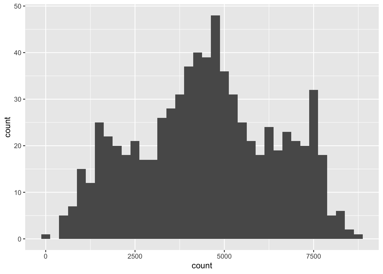
ggplot(bikeshare, aes(y = count, x = temp_orig)) +
  geom_point()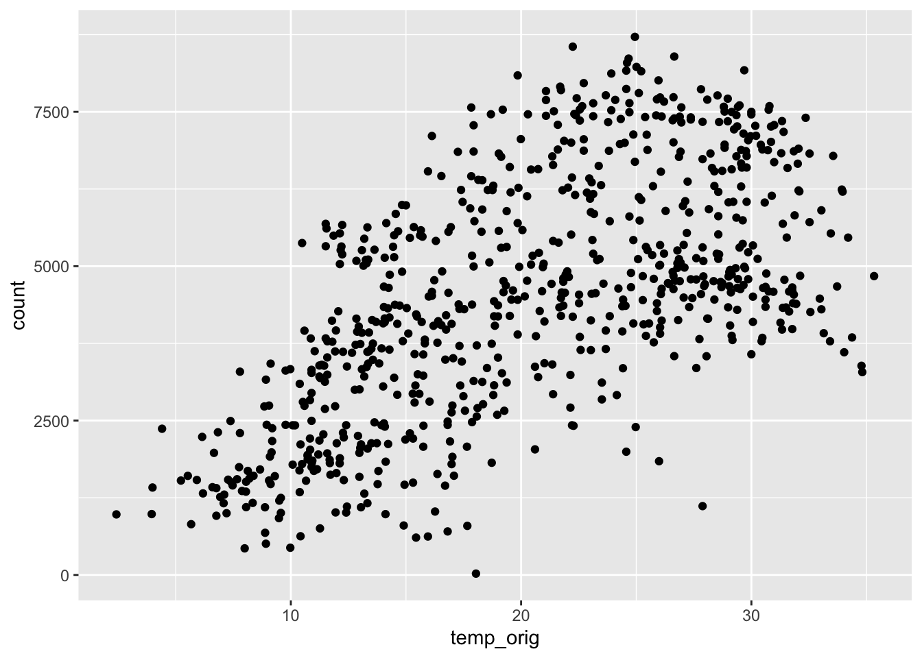
Exercise 2
Describe the distribution of daily bike rentals and the distribution of temperature based on the visualizations created in Exercise 1. Include the shape, center, spread, and presence of any potential outliers.
[Add your answer here]
Exercise 3
There appears to be one day with a very small number of bike rentals. What was the day? Why were the number of bike rentals so low on that day? Hint: You can Google the date to figure out what was going on that day.
[Add your answer here]
Exercise 4
Describe the relationship between daily bike rentals and temperature based on the visualization created in Exercise 1. Comment on how we expect the number of bike rentals to change as the temperature increases.
[Add your answer here]
Exercise 5
Suppose you want to fit a model so you can use the temperature to predict the number of bike rentals. Would a model of the form
\[\text{count} = \beta_0 + \beta_1 ~ \text{temp\_orig} + \epsilon\]
be the best fit for the data? Why or why not?
No.
Daily counts, temperature, and season
Exercise 6
In the raw data, seasons are coded as 1, 2, 3, 4 as numerical values, corresponding to winter, spring, summer, and fall respectively. Recode the season variable to make it a categorical variable (a factor) with levels corresponding to season names, making sure that the levels appear in a reasonable order in the variable (i.e., not alphabetical).
# add code developed during livecoding hereExercise 7
Next, let’s look at how the daily bike rentals differ by season. Let’s visualize the distribution of bike rentals by season using density plots. You can think of a density plot as a “smoothed out histogram”. Compare and contrast the distributions. Is this what you expected? Why or why not?
# add code developed during livecoding here[Add your answer here]
Exercise 8
We want to evaluate whether the relationship between temperature and daily bike rentals is the same for each season. To answer this question, first create a scatter plot of daily bike rentals vs. temperature faceted by season.
# add code developed during livecoding hereExercise 9
- Which season appears to have the strongest relationship between temperature and daily bike rentals? Why do you think the relationship is strongest in this season?
- Which season appears to have the weakest relationship between temperature and daily bike rentals? Why do you think the relationship is weakest in this season?
[Add your answer here]
Modeling
Exercise 10
Filter your data for the season with the strongest apparent relationship between temperature and daily bike rentals.
# add code developed during livecoding hereExercise 11
Using the data you filtered in Exercise 10, fit a linear model for predicting daily bike rentals from temperature for this season.
# add code developed during livecoding hereExercise 12
Use the output to write out the estimated regression equation.
[Add your answer here]
Exercise 13
Interpret the slope in the context of the data.
[Add your answer here]
Exercise 14
Interpret the intercept in the context of the data.
[Add your answer here]
Synthesis
Exercise 15
Suppose you work for a bike share company in Durham, NC, and they want to predict daily bike rentals in 2022. What is one reason you might recommend they use your analysis for this task? What is one reason you would recommend they not use your analysis for this task?
[Add your answer here]
The following exercises will be completed only if time permits.
Exercise 16
Pick another season. Based on the visualization in Exercise 8, would you expect the slope of the relationship between temperature and daily bike rentals to be smaller or larger than the slope of the model you’ve been working with so far? Explain your reasoning.
[Add your answer here]
Exercise 17
For this season you picked in Exercise 16, fit a linear model for predicting daily bike rentals from temperature. Note, you will need to filter your data for this season first. Use the output to write out the estimated regression equation and interpret the slope and the intercept of this model.
# add your code here[Add your answer here]