library(tidyverse)
library(tidymodels)
library(knitr)
library(colorblindr)AE 11: Multinomial classification
Important
Go to the course GitHub organization and locate the repo titled ae-11-volcanoes-YOUR_GITHUB_USERNAME to get started.
Packages
Data
For this application exercise we will work with a dataset of on volcanoes. The data come from The Smithsonian Institution via TidyTuesday.
volcano <- read_csv(here::here("ae", "data/volcano.csv"))Rows: 958 Columns: 26
── Column specification ────────────────────────────────────────────────────────
Delimiter: ","
chr (18): volcano_name, primary_volcano_type, last_eruption_year, country, r...
dbl (8): volcano_number, latitude, longitude, elevation, population_within_...
ℹ Use `spec()` to retrieve the full column specification for this data.
ℹ Specify the column types or set `show_col_types = FALSE` to quiet this message.First, a bit of data prep:
volcano <- volcano %>%
  mutate(
    volcano_type = case_when(
      str_detect(primary_volcano_type, "Stratovolcano") ~ "Stratovolcano",
      str_detect(primary_volcano_type, "Shield") ~ "Shield",
      TRUE ~ "Other"
    ),
    volcano_type = fct_relevel(volcano_type, "Stratovolcano", "Shield", "Other")
  ) %>%
  select(
    volcano_type, latitude, longitude,
    elevation, tectonic_settings, major_rock_1
    ) %>%
  mutate(across(where(is.character), as_factor))
Exploratory data analysis
- Create a map of volcanoes that is faceted by
volcano_type.
world <- map_data("world")

world_map <- ggplot() +
  geom_polygon(
    data = world,
    aes(
      x = long, y = lat, group = group),
      color = "white", fill = "gray50",
      size = 0.05, alpha = 0.2
    ) +
  theme_minimal() +
  coord_quickmap() +
  labs(x = NULL, y = NULL)

world_map +
  geom_point(
    data = volcano,
    aes(x = longitude, y = latitude,
        color = volcano_type,
        shape = volcano_type),
    alpha = 0.5
  ) +
  facet_wrap(~volcano_type) +
  scale_color_OkabeIto()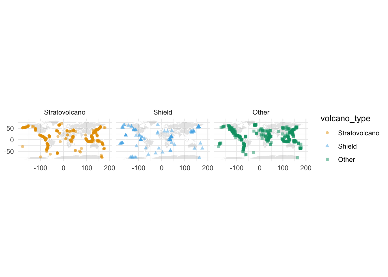
Build a new model
- Build a new model that uses a recipe that includes geographic information (latitude and longitude). How does this model compare to the original? Note:
Use the same test/train split as well as same cross validation folds. Code for these is provided below.
# test/train split
set.seed(1234)

volcano_split <- initial_split(volcano)
volcano_train <- training(volcano_split)
volcano_test  <- testing(volcano_split)

# cv folds
set.seed(9876)

volcano_folds <- vfold_cv(volcano_train, v = 5)
volcano_folds
# 5-fold cross-validation
# A tibble: 5 × 2
splits id
<list> <chr>
1 <split [574/144]> Fold1
2 <split [574/144]> Fold2
3 <split [574/144]> Fold3
4 <split [575/143]> Fold4
5 <split [575/143]> Fold5New recipe, including geographic information:
volcano_rec2 <- recipe(volcano_type ~ ., data = volcano_train) %>%
  step_other(tectonic_settings) %>%
  step_other(major_rock_1) %>%
  step_dummy(all_nominal_predictors()) %>%
  step_zv(all_predictors()) %>%
  step_center(all_predictors())
Original model specification and new workflow:
volcano_spec <- multinom_reg() %>%
  set_engine("nnet")

volcano_wflow2 <- workflow() %>%
  add_recipe(volcano_rec2) %>%
  add_model(volcano_spec)

volcano_wflow2
══ Workflow ════════════════════════════════════════════════════════════════════
Preprocessor: Recipe
Model: multinom_reg()
── Preprocessor ────────────────────────────────────────────────────────────────
5 Recipe Steps
• step_other()
• step_other()
• step_dummy()
• step_zv()
• step_center()
── Model ───────────────────────────────────────────────────────────────────────
Multinomial Regression Model Specification (classification)
Computational engine: nnet Fit resamples:
volcano_fit_rs2 <- volcano_wflow2 %>%
  fit_resamples(
    volcano_folds,
    control = control_resamples(save_pred = TRUE)
    )

volcano_fit_rs2
# Resampling results
# 5-fold cross-validation
# A tibble: 5 × 5
splits id .metrics .notes .predictions
<list> <chr> <list> <list> <list>
1 <split [574/144]> Fold1 <tibble [2 × 4]> <tibble [0 × 1]> <tibble [144 × 7]>
2 <split [574/144]> Fold2 <tibble [2 × 4]> <tibble [0 × 1]> <tibble [144 × 7]>
3 <split [574/144]> Fold3 <tibble [2 × 4]> <tibble [0 × 1]> <tibble [144 × 7]>
4 <split [575/143]> Fold4 <tibble [2 × 4]> <tibble [0 × 1]> <tibble [143 × 7]>
5 <split [575/143]> Fold5 <tibble [2 × 4]> <tibble [0 × 1]> <tibble [143 × 7]>Collect metrics:
collect_metrics(volcano_fit_rs2)# A tibble: 2 × 6
.metric .estimator mean n std_err .config
<chr> <chr> <dbl> <int> <dbl> <chr>
1 accuracy multiclass 0.606 5 0.0138 Preprocessor1_Model1
2 roc_auc hand_till 0.695 5 0.0245 Preprocessor1_Model1ROC curves:
volcano_fit_rs2 %>%
  collect_predictions() %>%
  group_by(id) %>%
  roc_curve(
    truth = volcano_type,
    .pred_Stratovolcano:.pred_Other
  ) %>%
  autoplot()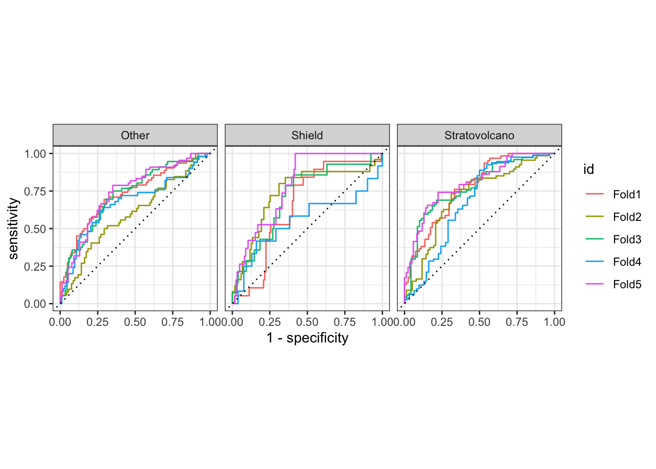
ROC curves
- Recreate the ROC curve from the slides.
final_fit <- last_fit(
  volcano_wflow2,
  split = volcano_split
  )

collect_predictions(final_fit) %>%
  roc_curve(truth = volcano_type, .pred_Stratovolcano:.pred_Other) %>%
  ggplot(aes(x = 1 - specificity, y = sensitivity, color = .level)) +
  geom_path(size = 1) +
  scale_color_OkabeIto() +
  geom_abline(intercept = 0, slope = 1, linetype = "dashed", color = "gray") +
  theme_minimal() +
  labs(color = NULL)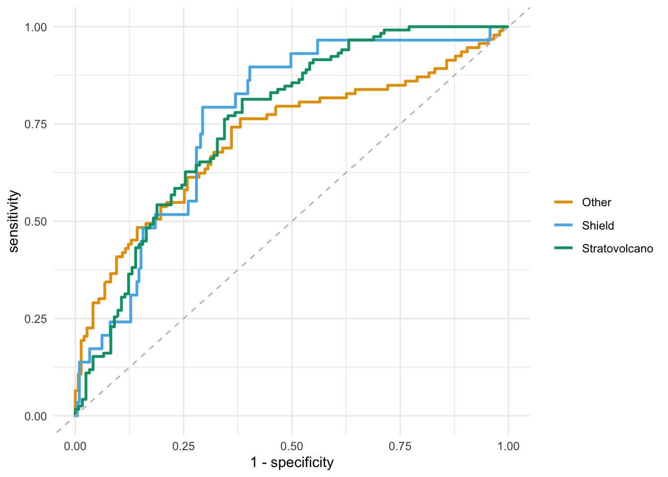
Acknowledgement
This exercise was inspired by https://juliasilge.com/blog/multinomial-volcano-eruptions.