MLR: Inference
STA 210 - Spring 2022
Welcome
Topics
Conduct a hypothesis test for \(\beta_j\)
Calculate a confidence interval for \(\beta_j\)
Inference pitfalls
Computational setup
Data: rail_trail
- The Pioneer Valley Planning Commission (PVPC) collected data for ninety days from April 5, 2005 to November 15, 2005.
- Data collectors set up a laser sensor, with breaks in the laser beam recording when a rail-trail user passed the data collection station.
# A tibble: 90 × 7
   volume hightemp avgtemp season cloudcover precip day_type
    <dbl>    <dbl>   <dbl> <chr>       <dbl>  <dbl> <chr>
 1    501       83    66.5 Summer       7.60 0      Weekday
 2    419       73    61   Summer       6.30 0.290  Weekday
 3    397       74    63   Spring       7.5  0.320  Weekday
 4    385       95    78   Summer       2.60 0      Weekend
 5    200       44    48   Spring      10    0.140  Weekday
 6    375       69    61.5 Spring       6.60 0.0200 Weekday
 7    417       66    52.5 Spring       2.40 0      Weekday
 8    629       66    52   Spring       0    0      Weekend
 9    533       80    67.5 Summer       3.80 0      Weekend
10    547       79    62   Summer       4.10 0      Weekday
# … with 80 more rows
Source: Pioneer Valley Planning Commission via the mosaicData package.
Variables
Outcome:
volume estimated number of trail users that day (number of breaks recorded)
Predictors
hightempdaily high temperature (in degrees Fahrenheit)avgtempaverage of daily low and daily high temperature (in degrees Fahrenheit)seasonone of “Fall”, “Spring”, or “Summer”cloudcovermeasure of cloud cover (in oktas)precipmeasure of precipitation (in inches)day_typeone of “weekday” or “weekend”
Conduct a hypothesis test for \(\beta_j\)
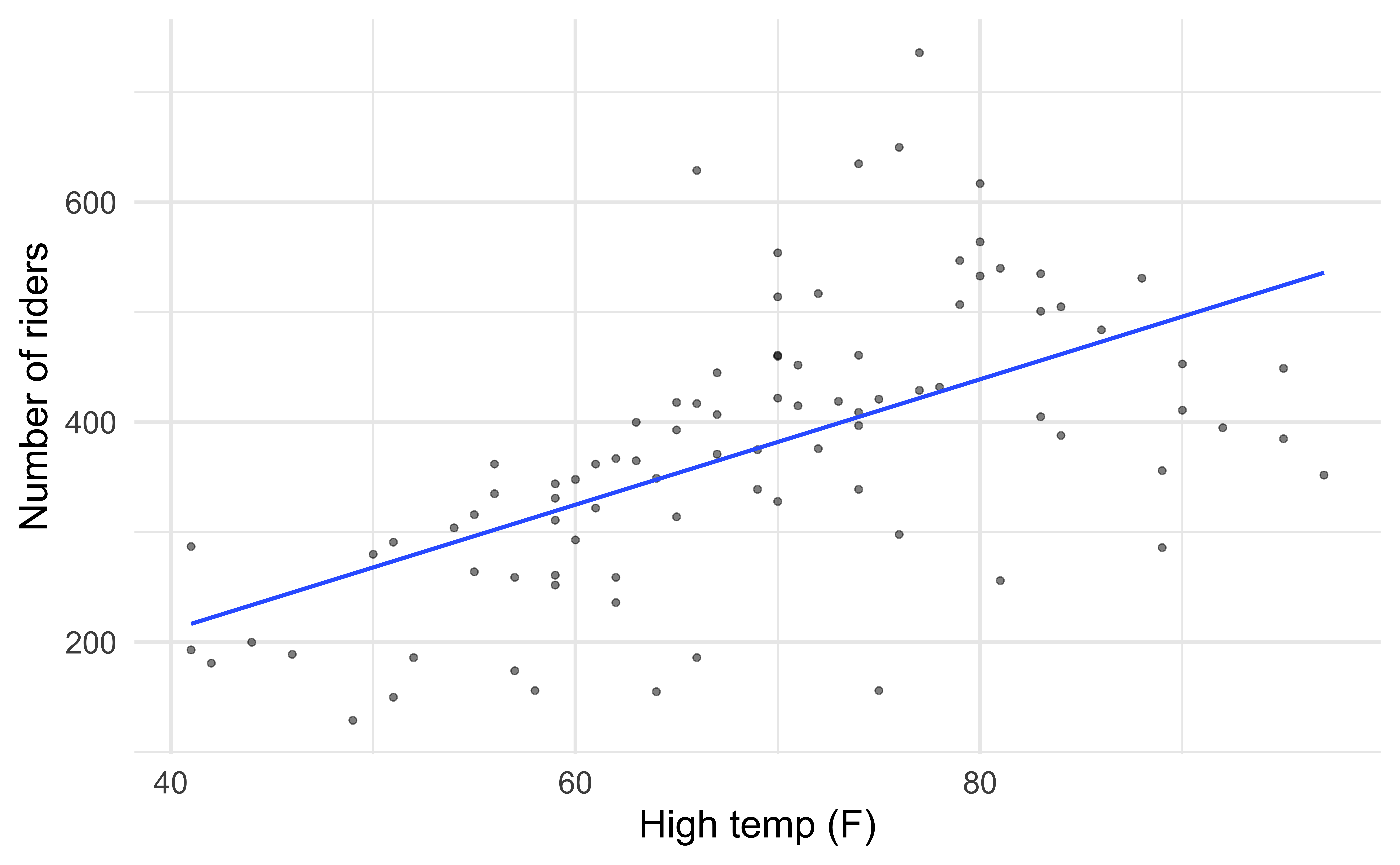
Review: Simple linear regression (SLR)

SLR model summary
SLR hypothesis test
# A tibble: 2 × 5
  term        estimate std.error statistic       p.value
  <chr>          <dbl>     <dbl>     <dbl>         <dbl>
1 (Intercept)   -17.1     59.4      -0.288 0.774
2 hightemp 5.70 0.848 6.72 0.00000000171- Set hypotheses: \(H_0: \beta_1 = 0\) and \(H_A: \beta_1 \ne 0\)
- Calculate test statistic and p-value: The test statistic is \(t = 6.72\) with a degrees of freedom of 88, and a p-value < 0.0001.
- State the conclusion: With a small p-value, we reject \(H_0\). The data provide strong evidence that high temperature is a helpful predictor for the number of daily riders.
Multiple linear regression
rt_mlr_main_fit <- linear_reg() %>%
  set_engine("lm") %>%
  fit(volume ~ hightemp + season, data = rail_trail)

tidy(rt_mlr_main_fit)
# A tibble: 4 × 5
term estimate std.error statistic p.value
<chr> <dbl> <dbl> <dbl> <dbl>
1 (Intercept) -125. 71.7 -1.75 0.0841
2 hightemp 7.54 1.17 6.43 0.00000000692
3 seasonSpring 5.13 34.3 0.150 0.881
4 seasonSummer -76.8 47.7 -1.61 0.111 MLR hypothesis test: hightemp
- Set hypotheses: \(H_0: \beta_{hightemp} = 0\) and \(H_A: \beta_{hightemp} \ne 0\), given
weekdayis in the model
- Calculate test statistic and p-value: The test statistic is \(t = 6.43\) with a degrees of freedom of 86, and a p-value < 0.0001.
- State the conclusion: With such a small p-value, the data provides strong evidence against \(H_0\), i.e., the data provide strong evidence that high temperature for the day is a helpful predictor in a model that already contains whether the given day is a weekday as a predictor for number of daily riders.
The model for season = Spring
| term | estimate | std.error | statistic | p.value |
|---|---|---|---|---|
| (Intercept) | -125.23 | 71.66 | -1.75 | 0.08 |
| hightemp | 7.54 | 1.17 | 6.43 | 0.00 |
| seasonSpring | 5.13 | 34.32 | 0.15 | 0.88 |
| seasonSummer | -76.84 | 47.71 | -1.61 | 0.11 |
\[ \begin{aligned} \widehat{volume} &= -125.23 + 7.54 \times \texttt{hightemp} + 5.13 \times \texttt{seasonSpring} - 76.84 \times \texttt{seasonSummer} \\ &= -125.23 + 7.54 \times \texttt{hightemp} + 5.13 \times 1 - 76.84 \times 0 \\ &= -120.10 + 7.54 \times \texttt{hightemp} \end{aligned} \]
The model for season = Summer
| term | estimate | std.error | statistic | p.value |
|---|---|---|---|---|
| (Intercept) | -125.23 | 71.66 | -1.75 | 0.08 |
| hightemp | 7.54 | 1.17 | 6.43 | 0.00 |
| seasonSpring | 5.13 | 34.32 | 0.15 | 0.88 |
| seasonSummer | -76.84 | 47.71 | -1.61 | 0.11 |
\[ \begin{aligned} \widehat{volume} &= -125.23 + 7.54 \times \texttt{hightemp} + 5.13 \times \texttt{seasonSpring} - 76.84 \times \texttt{seasonSummer} \\ &= -125.23 + 7.54 \times \texttt{hightemp} + 5.13 \times 0 - 76.84 \times 1 \\ &= -202.07 + 7.54 \times \texttt{hightemp} \end{aligned} \]
The model for season = Fall
| term | estimate | std.error | statistic | p.value |
|---|---|---|---|---|
| (Intercept) | -125.23 | 71.66 | -1.75 | 0.08 |
| hightemp | 7.54 | 1.17 | 6.43 | 0.00 |
| seasonSpring | 5.13 | 34.32 | 0.15 | 0.88 |
| seasonSummer | -76.84 | 47.71 | -1.61 | 0.11 |
\[ \begin{aligned} \widehat{volume} &= -125.23 + 7.54 \times \texttt{hightemp} + 5.13 \times \texttt{seasonSpring} - 76.84 \times \texttt{seasonSummer} \\ &= -125.23 + 7.54 \times \texttt{hightemp} + 5.13 \times 0 - 76.84 \times 0 \\ &= -125.23 + 7.54 \times \texttt{hightemp} \end{aligned} \]
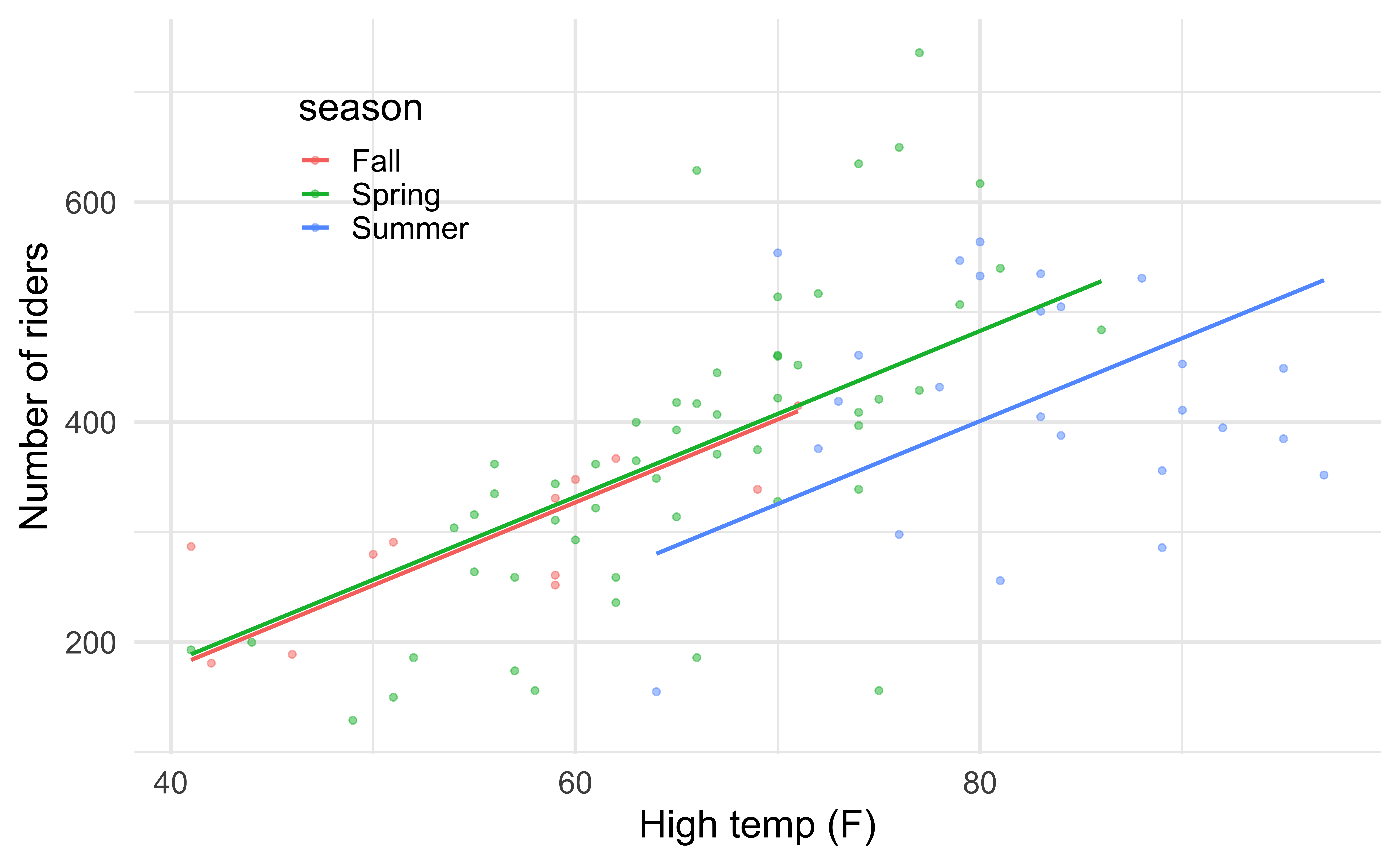
The models
Same slope, different intercepts
season = Spring: \(-120.10 + 7.54 \times \texttt{hightemp}\)season = Summer: \(-202.07 + 7.54 \times \texttt{hightemp}\)season = Fall: \(-125.23 + 7.54 \times \texttt{hightemp}\)
Application exercise
Ex 1. Recreate the following visualization in R based on the results of the model.

Application exercise
Ex 2. Add an interaction effect between hightemp and season and comment on the significance of the interaction predictors. Time permitting, visualize the interaction model as well.
10:00
Confidence interval for \(\beta_j\)
Confidence interval for \(\beta_j\)
The \(C%\) confidence interval for \(\beta_j\) \[\hat{\beta}_j \pm t^* SE(\hat{\beta}_j)\] where \(t^*\) follows a \(t\) distribution with \(n - p - 1\) degrees of freedom.
Generically, we are \(C%\) confident that the interval LB to UB contains the population coefficient of \(x_j\).
In context, we are \(C%\) confident that for every one unit increase in \(x_j\), we expect \(y\) to change by LB to UB units, holding all else constant.
Confidence interval for \(\beta_j\)
# A tibble: 4 × 7
  term         estimate std.error statistic       p.value conf.low conf.high
  <chr>           <dbl>     <dbl>     <dbl>         <dbl>    <dbl>     <dbl>
1 (Intercept)   -125.       71.7     -1.75  0.0841         -268.       17.2
2 hightemp         7.54      1.17     6.43  0.00000000692     5.21      9.87
3 seasonSpring     5.13     34.3      0.150 0.881           -63.1      73.4
4 seasonSummer   -76.8      47.7     -1.61  0.111          -172.       18.0
CI for hightemp
# A tibble: 4 × 7
  term         estimate std.error statistic       p.value conf.low conf.high
  <chr>           <dbl>     <dbl>     <dbl>         <dbl>    <dbl>     <dbl>
1 (Intercept)   -125.       71.7     -1.75  0.0841         -268.       17.2
2 hightemp         7.54      1.17     6.43  0.00000000692     5.21      9.87
3 seasonSpring     5.13     34.3      0.150 0.881           -63.1      73.4
4 seasonSummer   -76.8      47.7     -1.61  0.111          -172.       18.0
We are 95% confident that for every degrees Fahrenheit the day is warmer, we expect the number of riders to increase by 5.21 to 9.87, on average, holding season constant.
CI for seasonSpring
# A tibble: 4 × 7
  term         estimate std.error statistic       p.value conf.low conf.high
  <chr>           <dbl>     <dbl>     <dbl>         <dbl>    <dbl>     <dbl>
1 (Intercept)   -125.       71.7     -1.75  0.0841         -268.       17.2
2 hightemp         7.54      1.17     6.43  0.00000000692     5.21      9.87
3 seasonSpring     5.13     34.3      0.150 0.881           -63.1      73.4
4 seasonSummer   -76.8      47.7     -1.61  0.111          -172.       18.0
We are 95% confident that the number of riders on a Spring day is, on average, lower by 63.1 to higher by 73.4 compared to a Fall day, holding high temperature for the day constant.
Inference pitfalls
Large sample sizes
Danger
If the sample size is large enough, the test will likely result in rejecting \(H_0: \beta_j = 0\) even \(x_j\) has a very small effect on \(y\).
Consider the practical significance of the result not just the statistical significance.
Use the confidence interval to draw conclusions instead of relying only p-values.
Small sample sizes
Danger
If the sample size is small, there may not be enough evidence to reject \(H_0: \beta_j=0\).
When you fail to reject the null hypothesis, DON’T immediately conclude that the variable has no association with the response.
There may be a linear association that is just not strong enough to detect given your data, or there may be a non-linear association.
