Logistic regression

STA 210 - Spring 2022

Dr. Mine Çetinkaya-Rundel

Welcome

Announcements

Schedule changes for the remainder of the semester
Thursday office hours in my office: 213 Old Chem
Any questions on project proposals?

Topics

Logistic regression for binary response variable
Relationship between odds and probabilities
Use logistic regression model to calculate predicted odds and probabilities

Computational setup

# load packages
library(tidyverse)
library(tidymodels)
library(knitr)
library(Stat2Data)

# set default theme and larger font size for ggplot2
ggplot2::theme_set(ggplot2::theme_minimal(base_size = 20))

Predicting categorical outcomes

Types of outcome variables

Quantitative outcome variable:

Sales price of a house in Levittown, NY
Model: Expected sales price given the number of bedrooms, lot size, etc.

Categorical outcone variable:

High risk of coronary heart disease
Model: Probability an adult is high risk of heart disease given their age, total cholesterol, etc.

Models for categorical outcomes

Logistic regression

2 Outcomes

1: Yes, 0: No

Multinomial logistic regression

3+ Outcomes

1: Democrat, 2: Republican, 3: Independent

2020 election forecasts

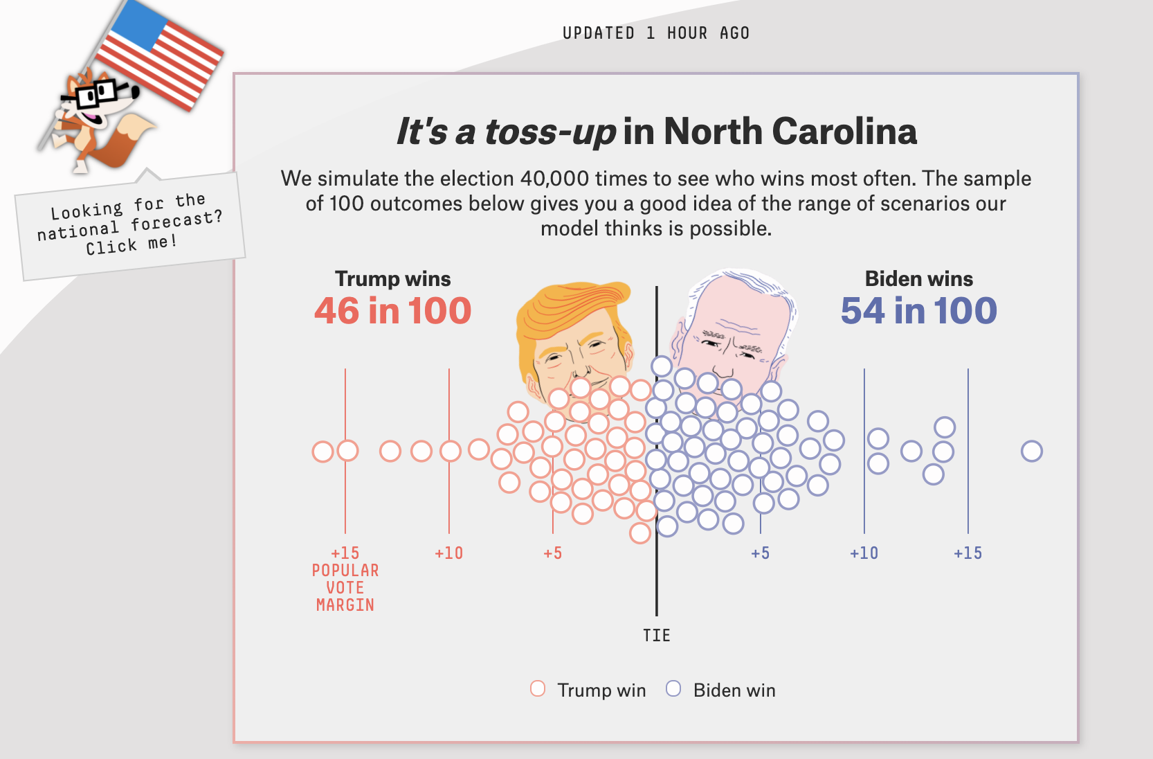
Source: FiveThirtyEight Election Forcasts

NBA finals predictions

Source: FiveThirtyEight 2019-20 NBA Predictions

Do teenagers get 7+ hours of sleep?

Students in grades 9 - 12 surveyed about health risk behaviors including whether they usually get 7 or more hours of sleep.

Sleep7

1: yes

0: no

data(YouthRisk2009)
sleep <- YouthRisk2009 %>%
  as_tibble() %>%
  filter(!is.na(Age), !is.na(Sleep7))
sleep %>%
  relocate(Age, Sleep7)

# A tibble: 446 × 6
     Age Sleep7 Sleep           SmokeLife SmokeDaily MarijuaEver
   <int>  <int> <fct>           <fct>     <fct>            <int>
 1    16      1 8 hours         Yes       Yes                  1
 2    17      0 5 hours         Yes       Yes                  1
 3    18      0 5 hours         Yes       Yes                  1
 4    17      1 7 hours         Yes       No                   1
 5    15      0 4 or less hours No        No                   0
 6    17      0 6 hours         No        No                   0
 7    17      1 7 hours         No        No                   0
 8    16      1 8 hours         Yes       No                   0
 9    16      1 8 hours         No        No                   0
10    18      0 4 or less hours Yes       Yes                  1
# … with 436 more rows

Plot the data

ggplot(sleep, aes(x = Age, y = Sleep7)) +
  geom_point() + 
  labs(y = "Getting 7+ hours of sleep")

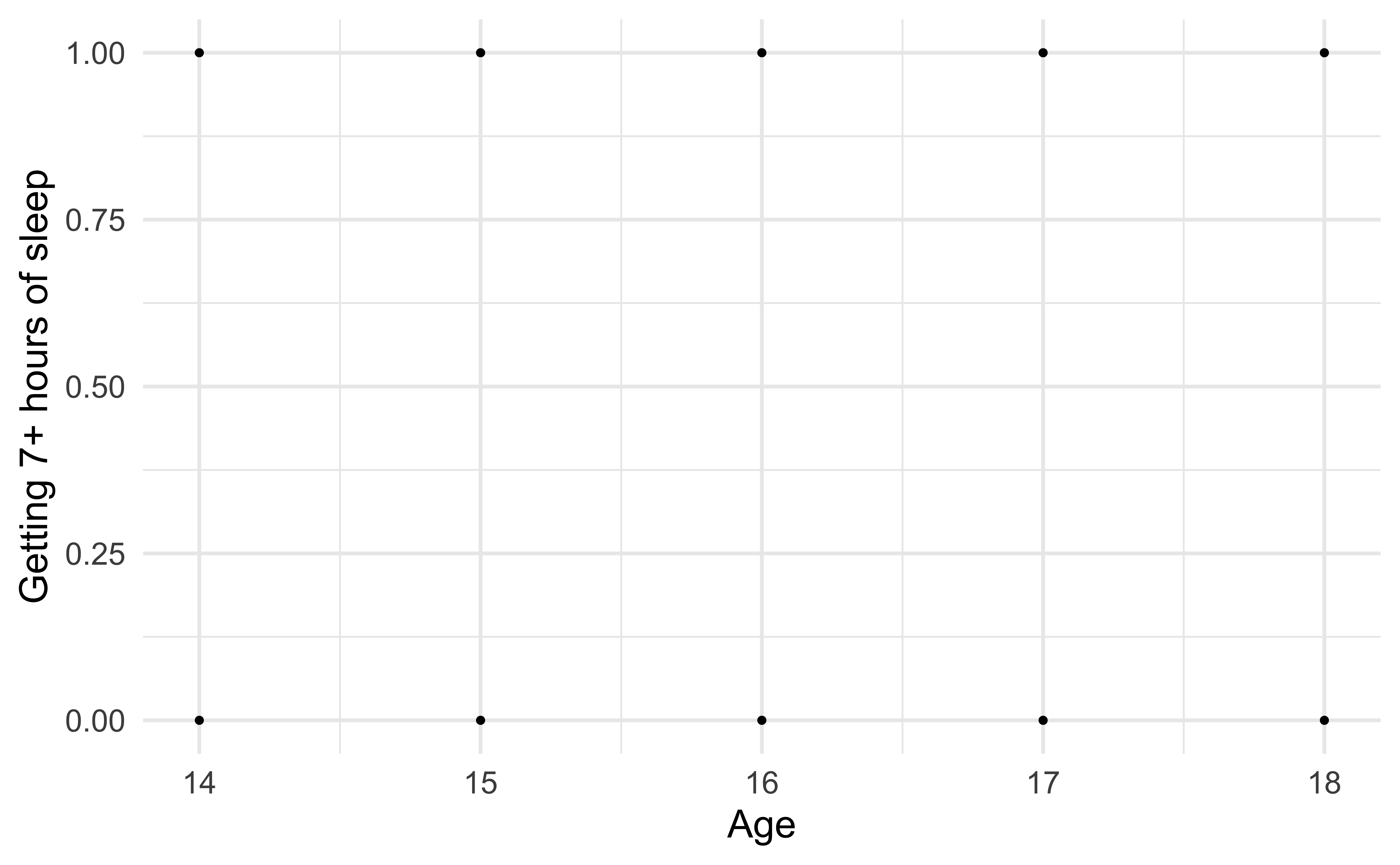
Let’s fit a linear regression model

Outcome: \(Y\) = 1: yes, 0: no

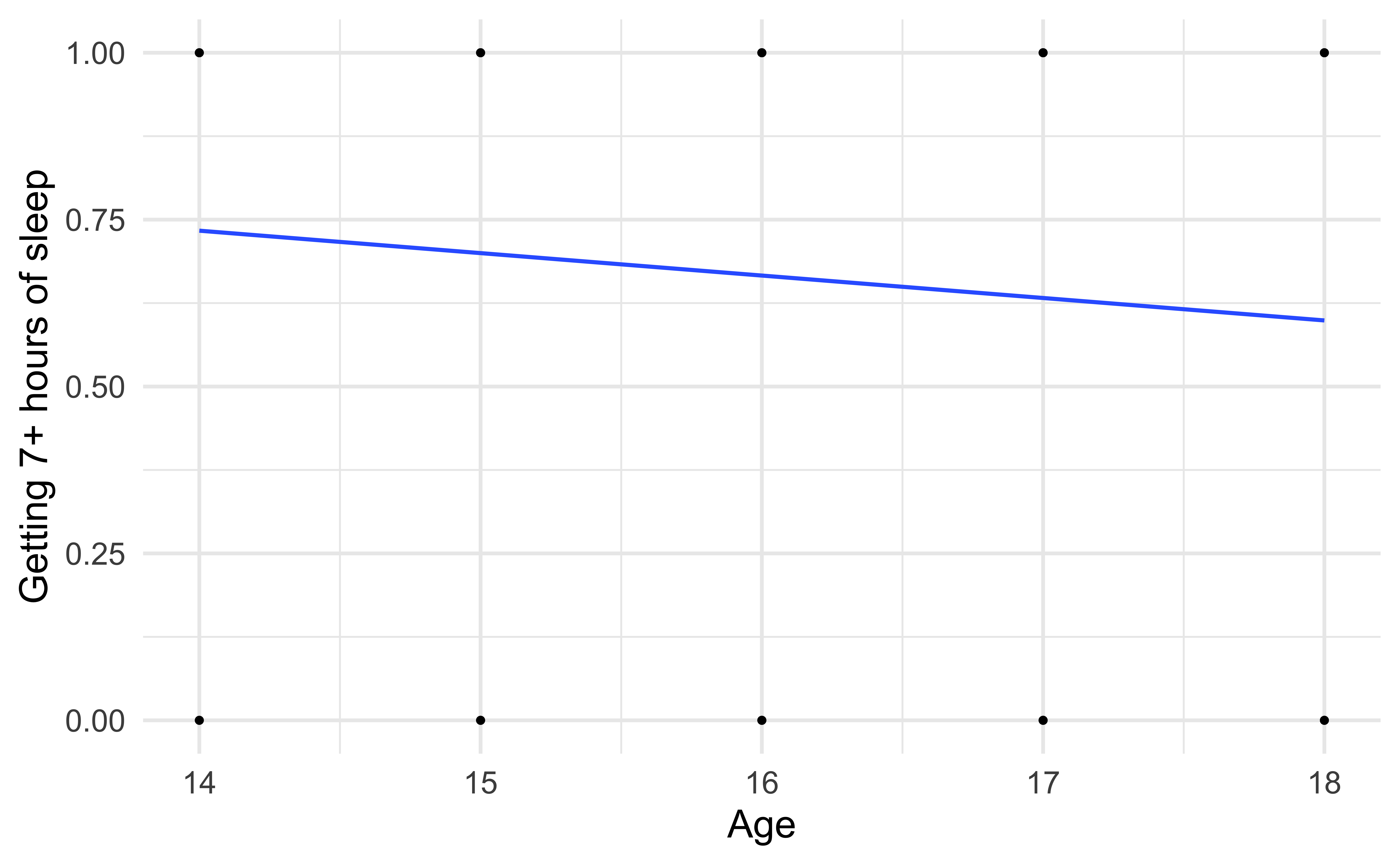
Let’s use proportions

Outcome: Probability of getting 7+ hours of sleep

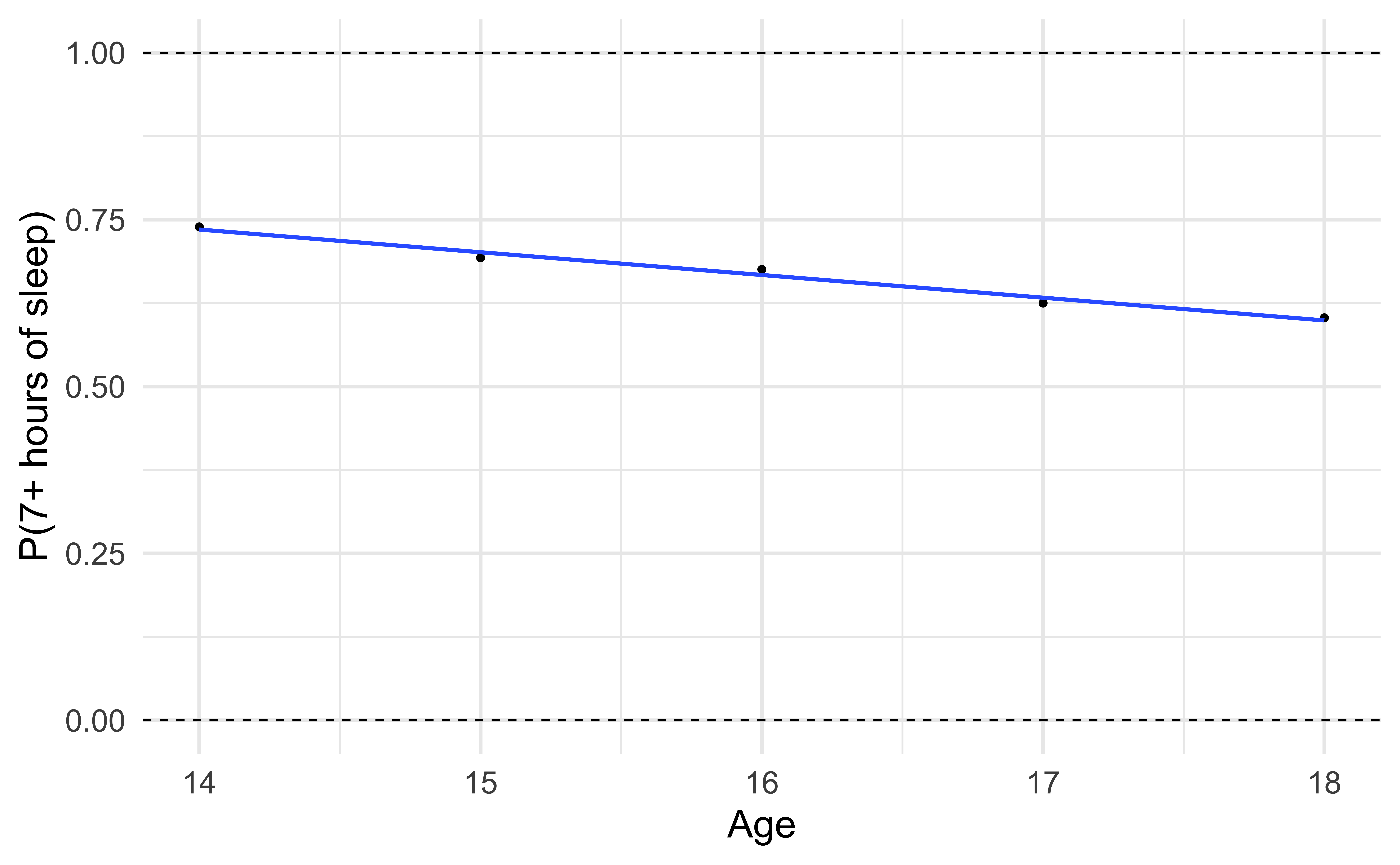
What happens if we zoom out?

Outcome: Probability of getting 7+ hours of sleep

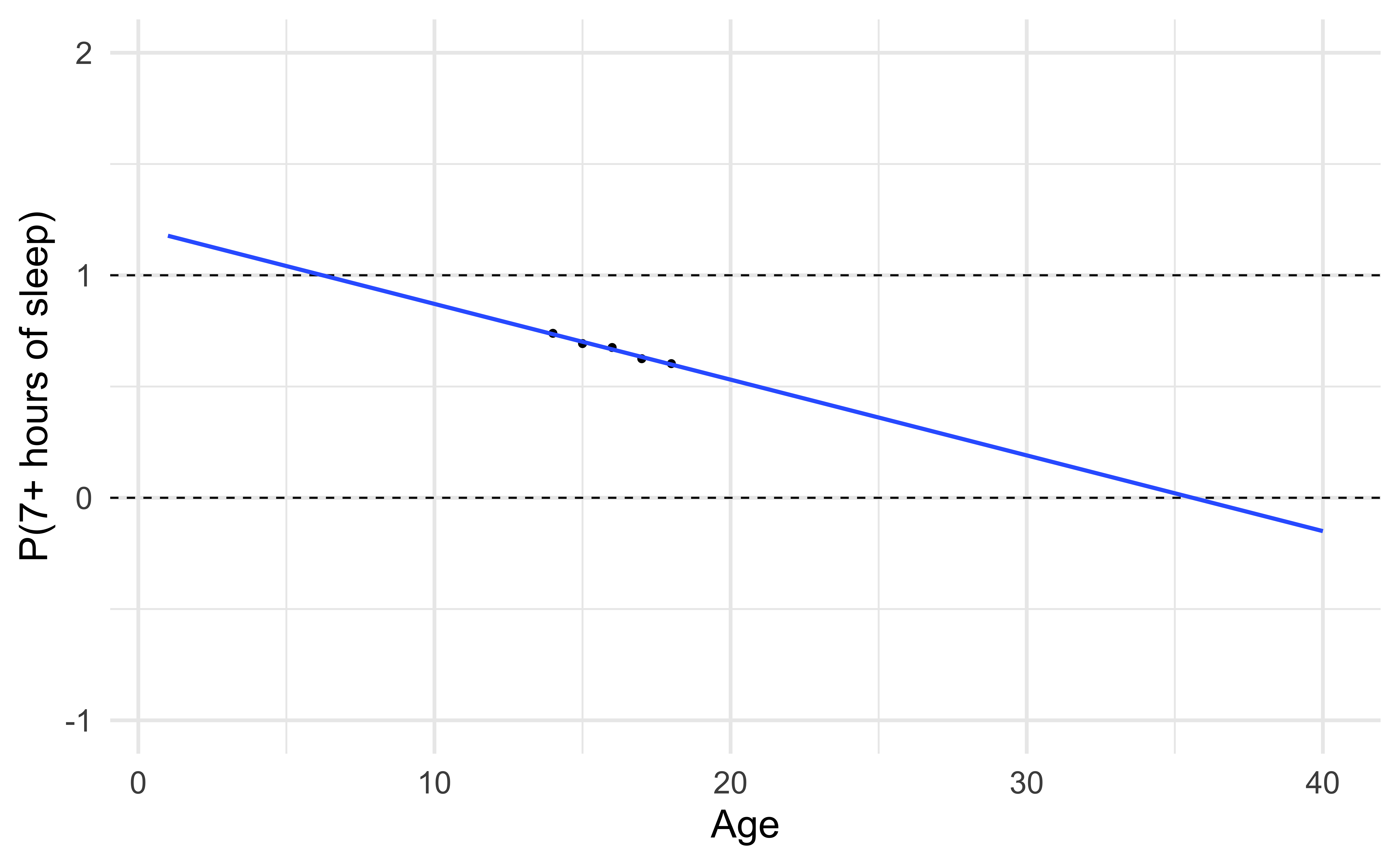
🛑 This model produces predictions outside of 0 and 1.

Let’s try another model

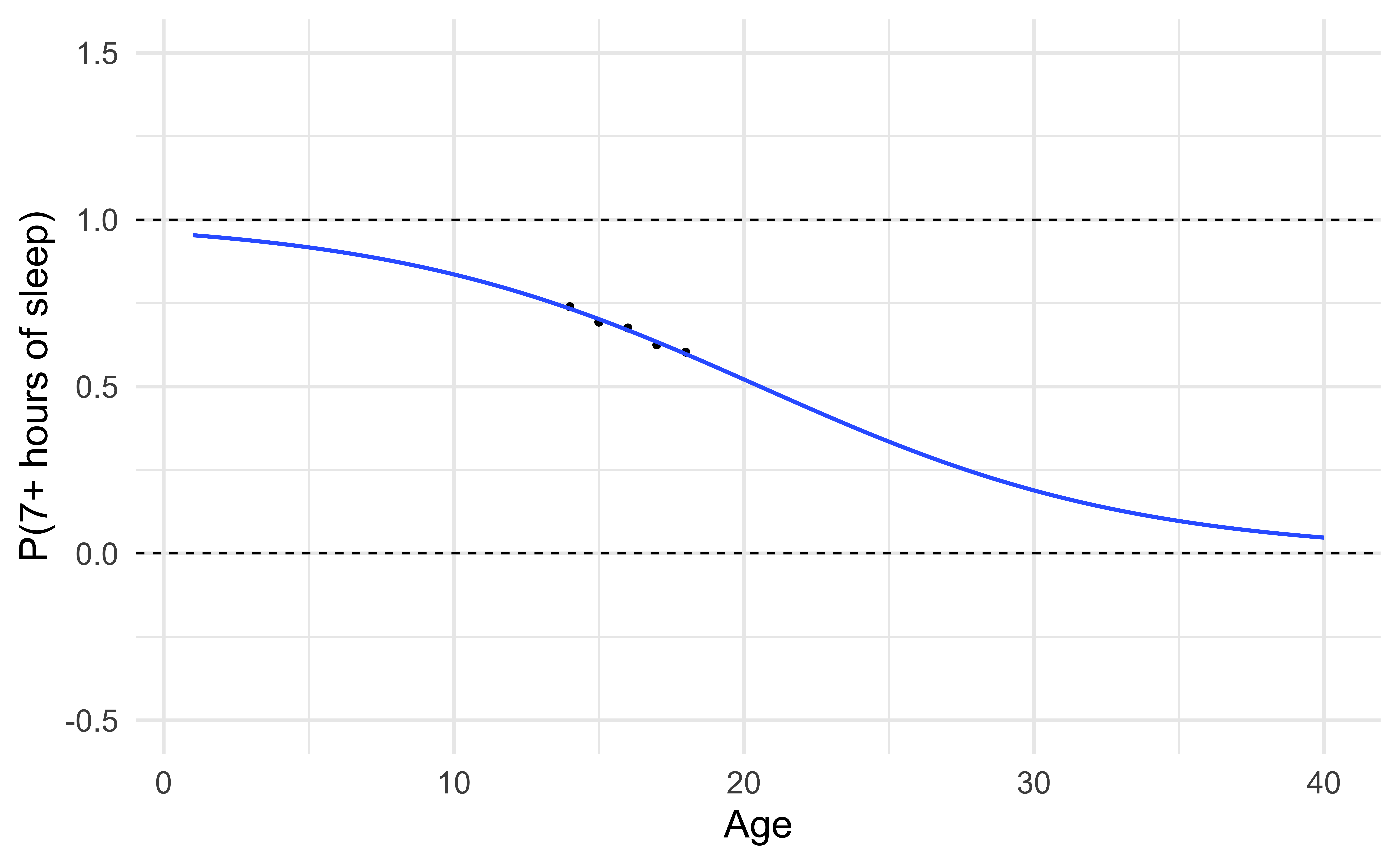
✅ This model (called a logistic regression model) only produces predictions between 0 and 1.

The code

ggplot(sleep_age, aes(x = Age, y = prop)) +
  geom_point() + 
  geom_hline(yintercept = c(0,1), lty = 2) + 
  stat_smooth(method ="glm", method.args = list(family = "binomial"), 
              fullrange = TRUE, se = FALSE) +
  labs(y = "P(7+ hours of sleep)") +
  xlim(1, 40) +
  ylim(-0.5, 1.5)

Different types of models

Method	Outcome	Model
Linear regression	Quantitative	\(Y = \beta_0 + \beta_1~ X\)
Linear regression (transform Y)	Quantitative	\(\log(Y) = \beta_0 + \beta_1~ X\)
Logistic regression	Binary	\(\log\big(\frac{\pi}{1-\pi}\big) = \beta_0 + \beta_1 ~ X\)

Odds and probabilities

Binary response variable

\(Y = 1: \text{ yes}, 0: \text{ no}\)
\(\pi\): probability that \(Y=1\), i.e., \(P(Y = 1)\)
\(\frac{\pi}{1-\pi}\): odds that \(Y = 1\)
\(\log\big(\frac{\pi}{1-\pi}\big)\): log odds
Go from \(\pi\) to \(\log\big(\frac{\pi}{1-\pi}\big)\) using the logit transformation

Odds

Suppose there is a 70% chance it will rain tomorrow

Probability it will rain is \(\mathbf{p = 0.7}\)
Probability it won’t rain is \(\mathbf{1 - p = 0.3}\)
Odds it will rain are 7 to 3, 7:3, \(\mathbf{\frac{0.7}{0.3} \approx 2.33}\)

Are teenagers getting enough sleep?

sleep %>%
  count(Sleep7) %>%
  mutate(p = round(n / sum(n), 3))

# A tibble: 2 × 3
  Sleep7     n     p
   <int> <int> <dbl>
1      0   150 0.336
2      1   296 0.664

\(P(\text{7+ hours of sleep}) = P(Y = 1) = p = 0.664\)

\(P(\text{< 7 hours of sleep}) = P(Y = 0) = 1 - p = 0.336\)

\(P(\text{odds of 7+ hours of sleep}) = \frac{0.664}{0.336} = 1.976\)

From odds to probabilities

odds

\[\omega = \frac{\pi}{1-\pi}\]

probability

\[\pi = \frac{\omega}{1 + \omega}\]

Logistic regression

From odds to probabilities

Logistic model: log odds = \(\log\big(\frac{\pi}{1-\pi}\big) = \beta_0 + \beta_1~X\)
Odds = \(\exp\big\{\log\big(\frac{\pi}{1-\pi}\big)\big\} = \frac{\pi}{1-\pi}\)
Combining (1) and (2) with what we saw earlier

\[\text{probability} = \pi = \frac{\exp\{\beta_0 + \beta_1~X\}}{1 + \exp\{\beta_0 + \beta_1~X\}}\]

Logistic regression model

Logit form: \[\log\big(\frac{\pi}{1-\pi}\big) = \beta_0 + \beta_1~X\]

Probability form:

\[ \pi = \frac{\exp\{\beta_0 + \beta_1~X\}}{1 + \exp\{\beta_0 + \beta_1~X\}} \]

Risk of coronary heart disease

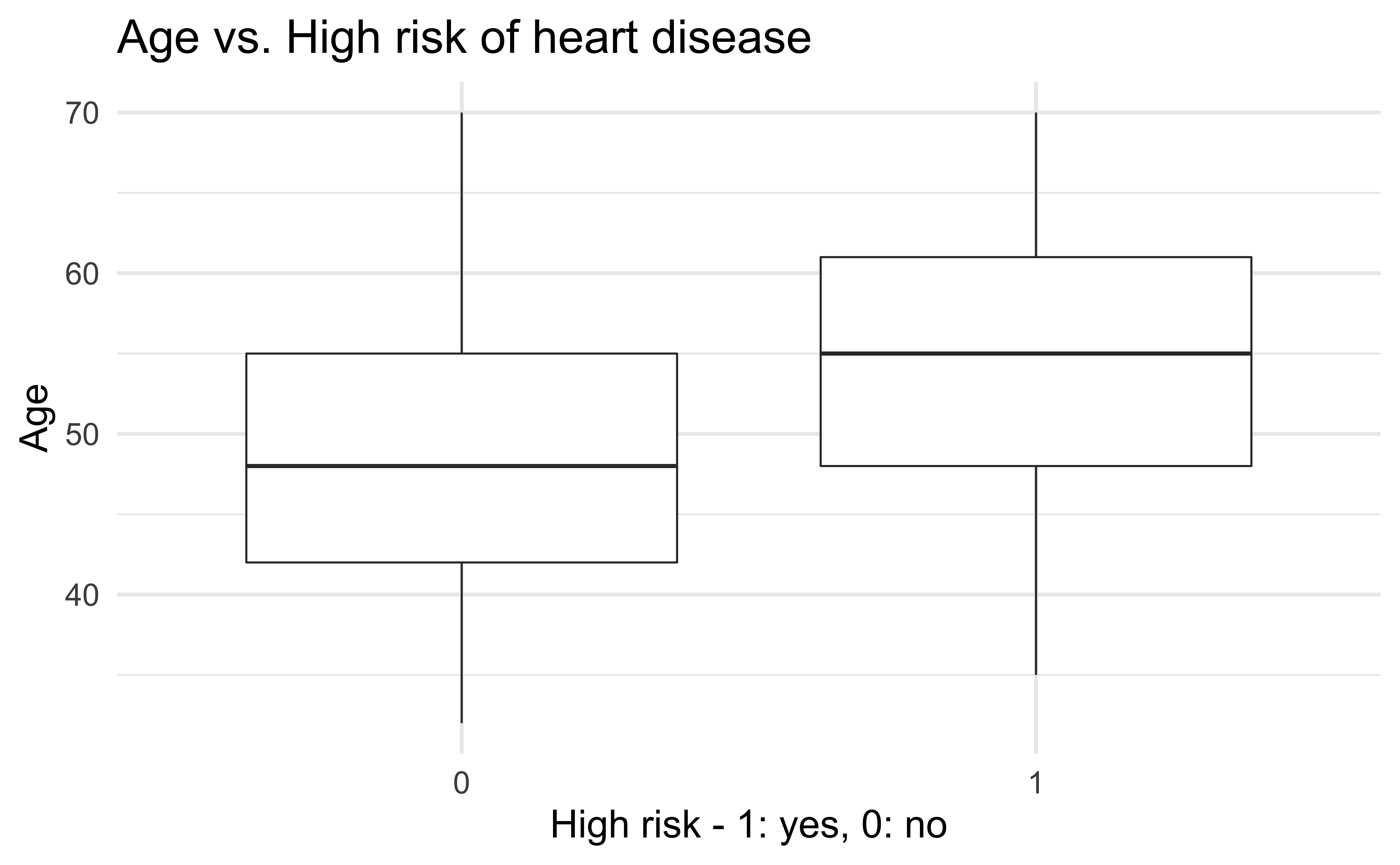
This dataset is from an ongoing cardiovascular study on residents of the town of Framingham, Massachusetts. We want to use age to predict if a randomly selected adult is high risk of having coronary heart disease in the next 10 years.

high_risk:

1: High risk of having heart disease in next 10 years
0: Not high risk of having heart disease in next 10 years

age: Age at exam time (in years)

Data: `heart`

heart_disease <- read_csv(here::here("slides", "data/framingham.csv")) %>%
  select(age, TenYearCHD) %>%
  drop_na() %>%
  mutate(high_risk = as.factor(TenYearCHD)) %>%
  select(age, high_risk)

heart_disease

# A tibble: 4,240 × 2
     age high_risk
   <dbl> <fct>    
 1    39 0        
 2    46 0        
 3    48 0        
 4    61 1        
 5    46 0        
 6    43 0        
 7    63 1        
 8    45 0        
 9    52 0        
10    43 0        
# … with 4,230 more rows

High risk vs. age

ggplot(heart_disease, aes(x = high_risk, y = age)) +
  geom_boxplot() +
  labs(x = "High risk - 1: yes, 0: no",
       y = "Age", 
       title = "Age vs. High risk of heart disease")

Let’s fit the model

heart_disease_fit <- logistic_reg() %>%
  set_engine("glm") %>%
  fit(high_risk ~ age, data = heart_disease, family = "binomial")

tidy(heart_disease_fit) %>% kable(digits = 3)

term	estimate	std.error	statistic	p.value
(Intercept)	-5.561	0.284	-19.599	0
age	0.075	0.005	14.178	0

The model

tidy(heart_disease_fit) %>% kable(digits = 3)

term	estimate	std.error	statistic	p.value
(Intercept)	-5.561	0.284	-19.599	0
age	0.075	0.005	14.178	0

. . .

\[\log\Big(\frac{\hat{\pi}}{1-\hat{\pi}}\Big) = -5.561 + 0.075 \times \text{age}\] where \(\hat{\pi}\) is the predicted probability of being high risk

Predicted log odds

augment(heart_disease_fit$fit)

# A tibble: 4,240 × 8
   high_risk   age .fitted .resid .std.resid     .hat .sigma   .cooksd
   <fct>     <dbl>   <dbl>  <dbl>      <dbl>    <dbl>  <dbl>     <dbl>
 1 0            39  -2.65  -0.370     -0.370 0.000466  0.895 0.0000165
 2 0            46  -2.13  -0.475     -0.475 0.000322  0.895 0.0000192
 3 0            48  -1.98  -0.509     -0.509 0.000288  0.895 0.0000199
 4 1            61  -1.01   1.62       1.62  0.000706  0.895 0.000968 
 5 0            46  -2.13  -0.475     -0.475 0.000322  0.895 0.0000192
 6 0            43  -2.35  -0.427     -0.427 0.000384  0.895 0.0000183
 7 1            63  -0.858  1.56       1.56  0.000956  0.895 0.00113  
 8 0            45  -2.20  -0.458     -0.458 0.000342  0.895 0.0000189
 9 0            52  -1.68  -0.585     -0.585 0.000262  0.895 0.0000244
10 0            43  -2.35  -0.427     -0.427 0.000384  0.895 0.0000183
# … with 4,230 more rows

For observation 1

\[\text{predicted odds} = \hat{\omega} = \frac{\hat{\pi}}{1-\hat{\pi}} = \exp\{-2.650\} = 0.071\]

Predicted probabilities

predict(heart_disease_fit, new_data = heart_disease, type = "prob")

# A tibble: 4,240 × 2
   .pred_0 .pred_1
     <dbl>   <dbl>
 1   0.934  0.0660
 2   0.894  0.106 
 3   0.878  0.122 
 4   0.733  0.267 
 5   0.894  0.106 
 6   0.913  0.0870
 7   0.702  0.298 
 8   0.900  0.0996
 9   0.843  0.157 
10   0.913  0.0870
# … with 4,230 more rows

\[\text{predicted probabilities} = \hat{\pi} = \frac{\exp\{-2.650\}}{1 + \exp\{-2.650\}} = 0.066\]

Predicted classes

predict(heart_disease_fit, new_data = heart_disease, type = "class")

# A tibble: 4,240 × 1
   .pred_class
   <fct>      
 1 0          
 2 0          
 3 0          
 4 0          
 5 0          
 6 0          
 7 0          
 8 0          
 9 0          
10 0          
# … with 4,230 more rows

Default prediction

For a logistic regression, the default prediction is the class.

predict(heart_disease_fit, new_data = heart_disease)

# A tibble: 4,240 × 1
   .pred_class
   <fct>      
 1 0          
 2 0          
 3 0          
 4 0          
 5 0          
 6 0          
 7 0          
 8 0          
 9 0          
10 0          
# … with 4,230 more rows

Observed vs. predicted

What does the following table show?

predict(heart_disease_fit, new_data = heart_disease) %>%
  bind_cols(heart_disease) %>%
  count(high_risk, .pred_class)

# A tibble: 2 × 3
  high_risk .pred_class     n
  <fct>     <fct>       <int>
1 0         0            3596
2 1         0             644

Recap

Logistic regression for binary response variable
Relationship between odds and probabilities
Used logistic regression model to calculate predicted odds and probabilities

Application exercise

📋 github.com/sta210-s22/ae-9-odds

Logistic regression

Welcome

Announcements

Topics

Computational setup

Predicting categorical outcomes

Types of outcome variables

Models for categorical outcomes

2020 election forecasts

NBA finals predictions

Do teenagers get 7+ hours of sleep?

Plot the data

Let’s fit a linear regression model

Let’s use proportions

What happens if we zoom out?

Let’s try another model

The code

Different types of models

Odds and probabilities

Binary response variable

Odds

Are teenagers getting enough sleep?

From odds to probabilities

Logistic regression

From odds to probabilities

Logistic regression model

Risk of coronary heart disease

Data: heart

High risk vs. age

Let’s fit the model

The model

Predicted log odds

Predicted probabilities

Predicted classes

Default prediction

Observed vs. predicted

Recap

Application exercise

Data: `heart`