MultiLR: Prediction + inferential models
STA 210 - Spring 2022
Welcome
Topics
- Predictions
- Model selection
- Checking conditions
Computational setup
NHANES Data
- National Health and Nutrition Examination Survey is conducted by the National Center for Health Statistics (NCHS).
- The goal is to “assess the health and nutritional status of adults and children in the United States”.
- This survey includes an interview and a physical examination.
Variables
Goal: Use a person’s age and whether they do regular physical activity to predict their self-reported health rating.
Outcome:
HealthGen: Self-reported rating of participant’s health in general. Excellent, Vgood, Good, Fair, or Poor.Predictors:
Age: Age at time of screening (in years). Participants 80 or older were recorded as 80.PhysActive: Participant does moderate to vigorous-intensity sports, fitness or recreational activities.
The data
Rows: 6,465
Columns: 5
$ HealthGen  <fct> Good, Good, Good, Good, Vgood, Vgood, Vgood, Vgood, Vgood, …
$ Age        <int> 34, 34, 34, 49, 45, 45, 45, 66, 58, 54, 50, 33, 60, 56, 56,…
$ PhysActive <fct> No, No, No, No, Yes, Yes, Yes, Yes, Yes, Yes, Yes, No, No, …
$ Education  <fct> High School, High School, High School, Some College, Colleg…
$ obs_num    <int> 1, 2, 3, 4, 5, 6, 7, 8, 9, 10, 11, 12, 13, 14, 15, 16, 17, …
Model in R
Model summary
# A tibble: 12 × 6
   y.level term            estimate std.error statistic  p.value
   <chr>   <chr>              <dbl>     <dbl>     <dbl>    <dbl>
 1 Vgood   (Intercept)    1.27        0.154      8.23   1.80e-16
 2 Vgood   Age           -0.0000361   0.00259   -0.0139 9.89e- 1
 3 Vgood   PhysActiveYes -0.332       0.0949    -3.50   4.72e- 4
 4 Good    (Intercept)    1.99        0.150     13.3    2.81e-40
 5 Good    Age           -0.00304     0.00256   -1.19   2.35e- 1
 6 Good    PhysActiveYes -1.01        0.0921   -11.0    4.80e-28
 7 Fair    (Intercept)    1.03        0.174      5.94   2.89e- 9
 8 Fair    Age            0.00113     0.00302    0.373  7.09e- 1
 9 Fair    PhysActiveYes -1.66        0.109    -15.2    4.14e-52
10 Poor    (Intercept)   -1.34        0.299     -4.47   7.65e- 6
11 Poor    Age            0.0193      0.00505    3.83   1.30e- 4
12 Poor    PhysActiveYes -2.67        0.236    -11.3    1.20e-29
Predictions
Calculating probabilities
For categories \(2,\ldots,K\), the probability that the \(i^{th}\) observation is in the \(j^{th}\) category is
\[ \hat{\pi}_{ij} = \frac{e^{\hat{\beta}_{0j} + \hat{\beta}_{1j}x_{i1} + \dots + \hat{\beta}_{pj}x_{ip}}}{1 + \sum\limits_{k=2}^K e^{\hat{\beta}_{0k} + \hat{\beta}_{1k}x_{i1} + \dots \hat{\beta}_{pk}x_{ip}}} \]
For the baseline category, \(k=1\), we calculate the probability \(\hat{\pi}_{i1}\) as
\[ \hat{\pi}_{i1} = 1- \sum\limits_{k=2}^K \hat{\pi}_{ik} \]
Predicted health rating
We can use our model to predict a person’s perceived health rating given their age and whether they exercise.
# A tibble: 6,465 × 11
   HealthGen   Age PhysActive Education      obs_num .pred_class .pred_Excellent
   <fct>     <int> <fct>      <fct>            <int> <fct>                 <dbl>
 1 Good         34 No         High School          1 Good                 0.0687
 2 Good         34 No         High School          2 Good                 0.0687
 3 Good         34 No         High School          3 Good                 0.0687
 4 Good         49 No         Some College         4 Good                 0.0691
 5 Vgood        45 Yes        College Grad         5 Vgood                0.155
 6 Vgood        45 Yes        College Grad         6 Vgood                0.155
 7 Vgood        45 Yes        College Grad         7 Vgood                0.155
 8 Vgood        66 Yes        Some College         8 Vgood                0.157
 9 Vgood        58 Yes        College Grad         9 Vgood                0.156
10 Fair         54 Yes        9 - 11th Grade      10 Vgood                0.156
# … with 6,455 more rows, and 4 more variables: .pred_Vgood <dbl>,
#   .pred_Good <dbl>, .pred_Fair <dbl>, .pred_Poor <dbl>
Actual vs. predicted health rating
For each observation, the predicted perceived health rating is the category with the highest predicted probability.
# A tibble: 6,465 × 6
   .pred_class .pred_Excellent .pred_Vgood .pred_Good .pred_Fair .pred_Poor
   <fct>                 <dbl>       <dbl>      <dbl>      <dbl>      <dbl>
 1 Good                 0.0687       0.243      0.453     0.201     0.0348
 2 Good                 0.0687       0.243      0.453     0.201     0.0348
 3 Good                 0.0687       0.243      0.453     0.201     0.0348
 4 Good                 0.0691       0.244      0.435     0.205     0.0467
 5 Vgood                0.155        0.393      0.359     0.0868    0.00671
 6 Vgood                0.155        0.393      0.359     0.0868    0.00671
 7 Vgood                0.155        0.393      0.359     0.0868    0.00671
 8 Vgood                0.157        0.400      0.342     0.0904    0.0102
 9 Vgood                0.156        0.397      0.349     0.0890    0.00872
10 Vgood                0.156        0.396      0.352     0.0883    0.00804
# … with 6,455 more rows
Confusion matrix
health_conf <- health_aug %>%
  count(HealthGen, .pred_class, .drop = FALSE) %>%
  pivot_wider(names_from = .pred_class, values_from = n)

health_conf
# A tibble: 5 × 6
HealthGen Excellent Vgood Good Fair Poor
<fct> <int> <int> <int> <int> <int>
1 Excellent 0 528 210 0 0
2 Vgood 0 1341 743 0 0
3 Good 0 1226 1316 0 0
4 Fair 0 296 625 0 0
5 Poor 0 24 156 0 0Actual vs. predicted health rating
Why do you think no observations were predicted to have a rating of “Excellent”, “Fair”, or “Poor”?
Model selection for inference
Comparing nested models
- Suppose there are two models:
- Reduced model includes predictors \(x_1, \ldots, x_q\)
- Full model includes predictors \(x_1, \ldots, x_q, x_{q+1}, \ldots, x_p\)
- We want to test the following hypotheses:
- \(H_0: \beta_{q+1} = \dots = \beta_p = 0\)
- \(H_A: \text{ at least 1 }\beta_j \text{ is not } 0\)
- To do so, we will use the drop-in-deviance test (very similar to logistic regression)
Add Education to the model?
- We consider adding the participants’
Educationlevel to the model.- Education takes values
8thGrade,9-11thGrade,HighSchool,SomeCollege, andCollegeGrad
- Education takes values
- Models we’re testing:
- Reduced model:
Age,PhysActive - Full model:
Age,PhysActive,Education
- Reduced model:
\[ \begin{align} &H_0: \beta_{9-11thGrade} = \beta_{HighSchool} = \beta_{SomeCollege} = \beta_{CollegeGrad} = 0\\ &H_a: \text{ at least one }\beta_j \text{ is not equal to }0 \end{align} \]
Add Education to the model?
reduced_fit <- multinom_reg() %>%
  set_engine("nnet") %>%
  fit(HealthGen ~ Age + PhysActive,
  data = nhanes_adult)

full_fit <- multinom_reg() %>%
  set_engine("nnet") %>%
  fit(HealthGen ~ Age + PhysActive + Education,
  data = nhanes_adult)

reduced_fit <- repair_call(reduced_fit, data = nhanes_adult)
full_fit <- repair_call(full_fit, data = nhanes_adult)
Add Education to the model?
| Model | Resid. df | Resid. Dev | Test | Df | LR stat. | Pr(Chi) |
|---|---|---|---|---|---|---|
| Age + PhysActive | 25848 | 16994.23 | NA | NA | NA | |
| Age + PhysActive + Education | 25832 | 16505.10 | 1 vs 2 | 16 | 489.132 | 0 |
At least one coefficient associated with Education is non-zero. Therefore, we will include Education in the model.
Model with Education
# A tibble: 28 × 8
   y.level term         estimate std.error statistic  p.value conf.low conf.high
   <chr>   <chr>           <dbl>     <dbl>     <dbl>    <dbl>    <dbl>     <dbl>
 1 Vgood   (Intercept)   5.82e-1   0.301      1.93   5.36e- 2 -0.00914   1.17
 2 Vgood   Age           1.12e-3   0.00266    0.419  6.75e- 1 -0.00411   0.00634
 3 Vgood   PhysActiveY… -2.64e-1   0.0985    -2.68   7.33e- 3 -0.457    -0.0711
 4 Vgood   Education9 …  7.68e-1   0.308      2.49   1.27e- 2  0.164     1.37
 5 Vgood   EducationHi…  7.01e-1   0.280      2.51   1.21e- 2  0.153     1.25
 6 Vgood   EducationSo…  7.88e-1   0.271      2.90   3.71e- 3  0.256     1.32
 7 Vgood   EducationCo…  4.08e-1   0.268      1.52   1.28e- 1 -0.117     0.933
 8 Good    (Intercept)   2.04e+0   0.272      7.51   5.77e-14  1.51      2.57
 9 Good    Age          -1.72e-3   0.00263   -0.651  5.15e- 1 -0.00688   0.00345
10 Good    PhysActiveY… -7.58e-1   0.0961    -7.88   3.16e-15 -0.946    -0.569
11 Good    Education9 …  3.60e-1   0.275      1.31   1.90e- 1 -0.179     0.899
12 Good    EducationHi…  8.52e-2   0.247      0.345  7.30e- 1 -0.399     0.569
13 Good    EducationSo… -1.13e-2   0.239     -0.0472 9.62e- 1 -0.480     0.457
14 Good    EducationCo… -8.91e-1   0.236     -3.77   1.65e- 4 -1.35     -0.427
15 Fair    (Intercept)   2.12e+0   0.288      7.35   1.91e-13  1.55      2.68
16 Fair    Age           3.35e-4   0.00312    0.107  9.14e- 1 -0.00578   0.00645
17 Fair    PhysActiveY… -1.19e+0   0.115    -10.4    3.50e-25 -1.42     -0.966
18 Fair    Education9 … -2.24e-1   0.279     -0.802  4.22e- 1 -0.771     0.323
19 Fair    EducationHi… -8.32e-1   0.252     -3.31   9.44e- 4 -1.33     -0.339
20 Fair    EducationSo… -1.34e+0   0.246     -5.46   4.71e- 8 -1.82     -0.861
21 Fair    EducationCo… -2.51e+0   0.253     -9.91   3.67e-23 -3.00     -2.01
22 Poor    (Intercept)  -2.00e-1   0.411     -0.488  6.26e- 1 -1.01      0.605
23 Poor    Age           1.79e-2   0.00509    3.53   4.21e- 4  0.00797   0.0279
24 Poor    PhysActiveY… -2.27e+0   0.242     -9.38   6.81e-21 -2.74     -1.79
25 Poor    Education9 … -3.60e-1   0.353     -1.02   3.08e- 1 -1.05      0.332
26 Poor    EducationHi… -1.15e+0   0.334     -3.44   5.86e- 4 -1.81     -0.494
27 Poor    EducationSo… -1.07e+0   0.316     -3.40   6.77e- 4 -1.69     -0.454
28 Poor    EducationCo… -2.32e+0   0.366     -6.34   2.27e-10 -3.04     -1.60
Compare NHANES models using AIC
Reduced model:
Checking conditions for inference
Conditions for inference
We want to check the following conditions for inference for the multinomial logistic regression model:
Linearity: Is there a linear relationship between the log-odds and the predictor variables?
Randomness: Was the sample randomly selected? Or can we reasonably treat it as random?
Independence: Are the observations independent?
Checking linearity
Similar to logistic regression, we will check linearity by examining empirical logit plots between each level of the response and the quantitative predictor variables.
nhanes_adult <- nhanes_adult %>%
  mutate(
    Excellent = factor(if_else(HealthGen == "Excellent", "1", "0")),
    Vgood = factor(if_else(HealthGen == "Vgood", "1", "0")),
    Good = factor(if_else(HealthGen == "Good", "1", "0")),
    Fair = factor(if_else(HealthGen == "Fair", "1", "0")),
    Poor = factor(if_else(HealthGen == "Poor", "1", "0"))
  )
Checking linearity
Checking linearity
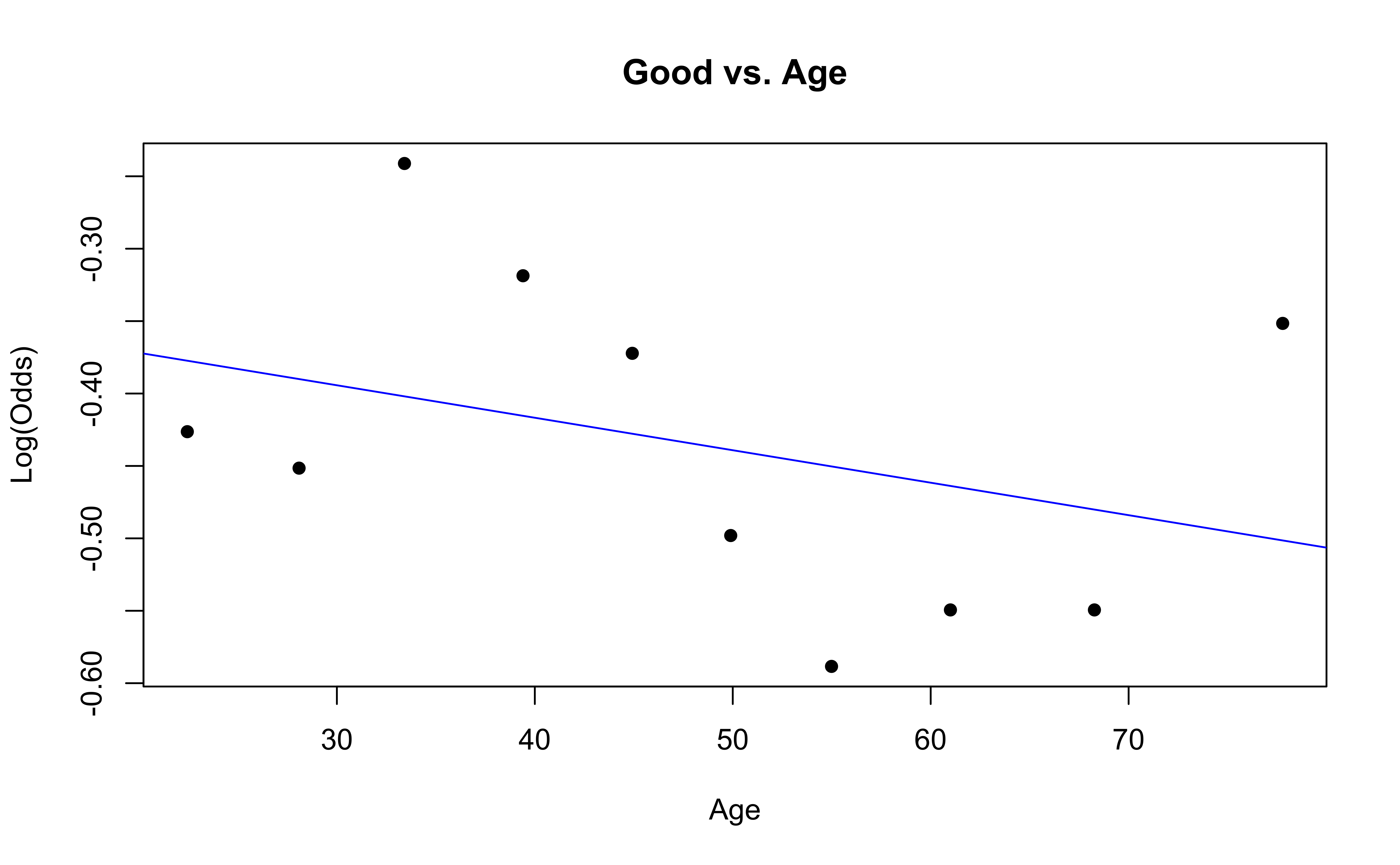
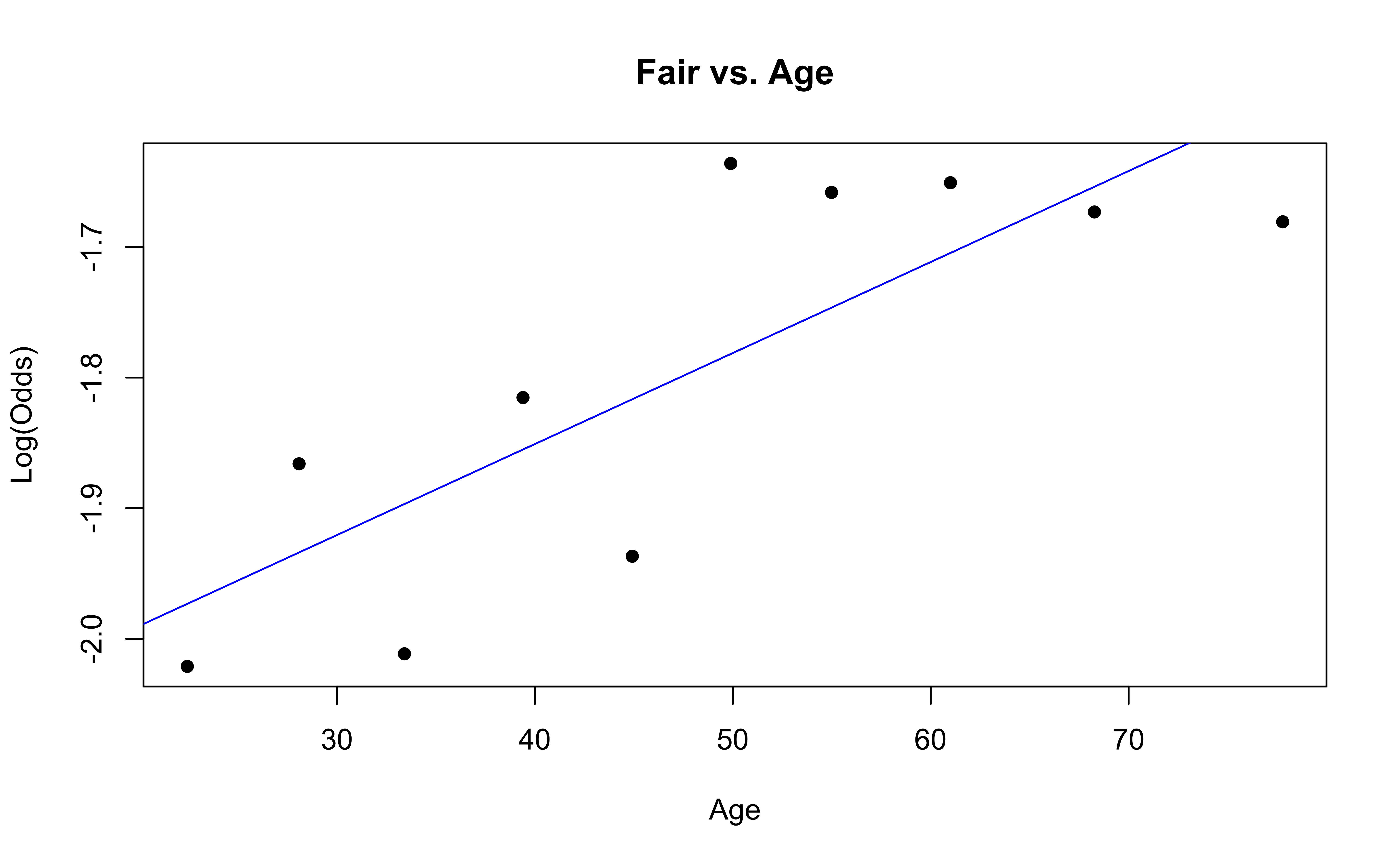
Checking linearity
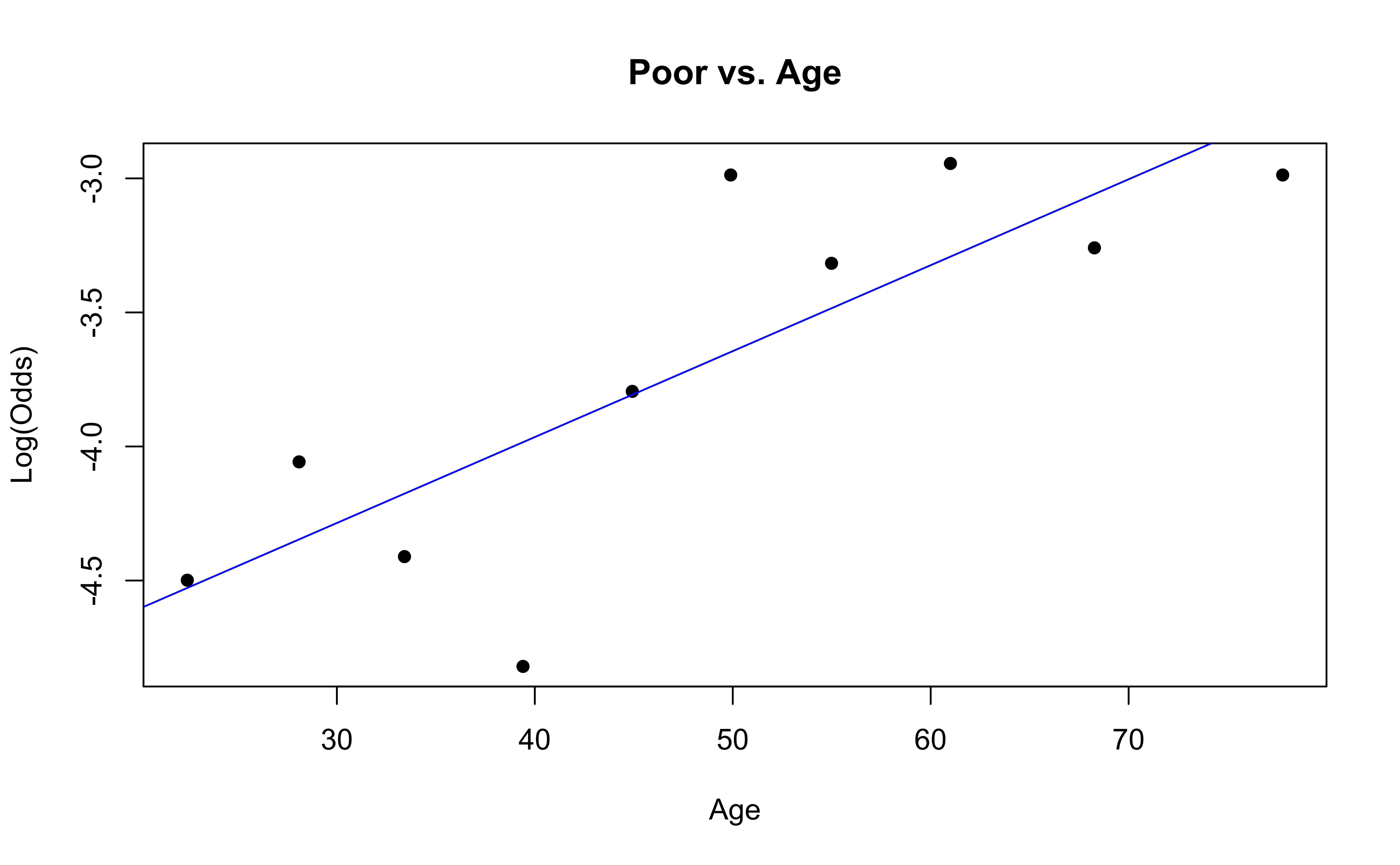
✅ The linearity condition is satisfied. There is a linear relationship between the empirical logit and the quantitative predictor variable, Age.
Checking randomness
We can check the randomness condition based on the context of the data and how the observations were collected.
Was the sample randomly selected?
If the sample was not randomly selected, ask whether there is reason to believe the observations in the sample differ systematically from the population of interest.
✅ The randomness condition is satisfied. We do not have reason to believe that the participants in this study differ systematically from adults in the U.S..
Checking independence
We can check the independence condition based on the context of the data and how the observations were collected.
Independence is most often violated if the data were collected over time or there is a strong spatial relationship between the observations.
✅ The independence condition is satisfied. It is reasonable to conclude that the participants’ health and behavior characteristics are independent of one another.
Recap
- Predictions
- Model selection for inference
- Checking conditions for inference