SLR: Model fitting in R with tidymodels

STA 210 - Spring 2022

Dr. Mine Çetinkaya-Rundel

Welcome

Announcements

• If you’re just joining the class, welcome! Go to the course website and review content you’ve missed, read the syllabus, and complete the Getting to know you survey.
• Lab 1 is due Friday, at 5pm, on Gradescope.

Recap of last lecture

• Used simple linear regression to describe the relationship between a quantitative predictor and quantitative outcome variable.

• Used the least squares method to estimate the slope and intercept.

• We interpreted the slope and intercept.

  • Slope: For every one unit increase in \(x\), we expect y to be higher/lower by \(\hat{\beta}_1\) units, on average.
  • Intercept: If \(x\) is 0, then we expect \(y\) to be \(\hat{\beta}_0\) units.

• Predicted the response given a value of the predictor variable.

• Defined extrapolation and why we should avoid it.

Interested in the math behind it all?

See the supplemental notes on Deriving the Least-Squares Estimates for Simple Linear Regression for more mathematical details on the derivations of the estimates of \(\beta_0\) and \(\beta_1\).

Outline

• Use tidymodels to fit and summarize regression models in R
• Complete an application exercise on exploratory data analysis and modeling

Computational setup

# load packages
library(tidyverse)       # for data wrangling
library(tidymodels)      # for modeling
library(fivethirtyeight) # for the fandango dataset

# set default theme and larger font size for ggplot2
ggplot2::theme_set(ggplot2::theme_minimal(base_size = 16))

# set default figure parameters for knitr
knitr::opts_chunk$set(
  fig.width = 8,
  fig.asp = 0.618,
  fig.retina = 3,
  dpi = 300,
  out.width = "80%"
)

Data

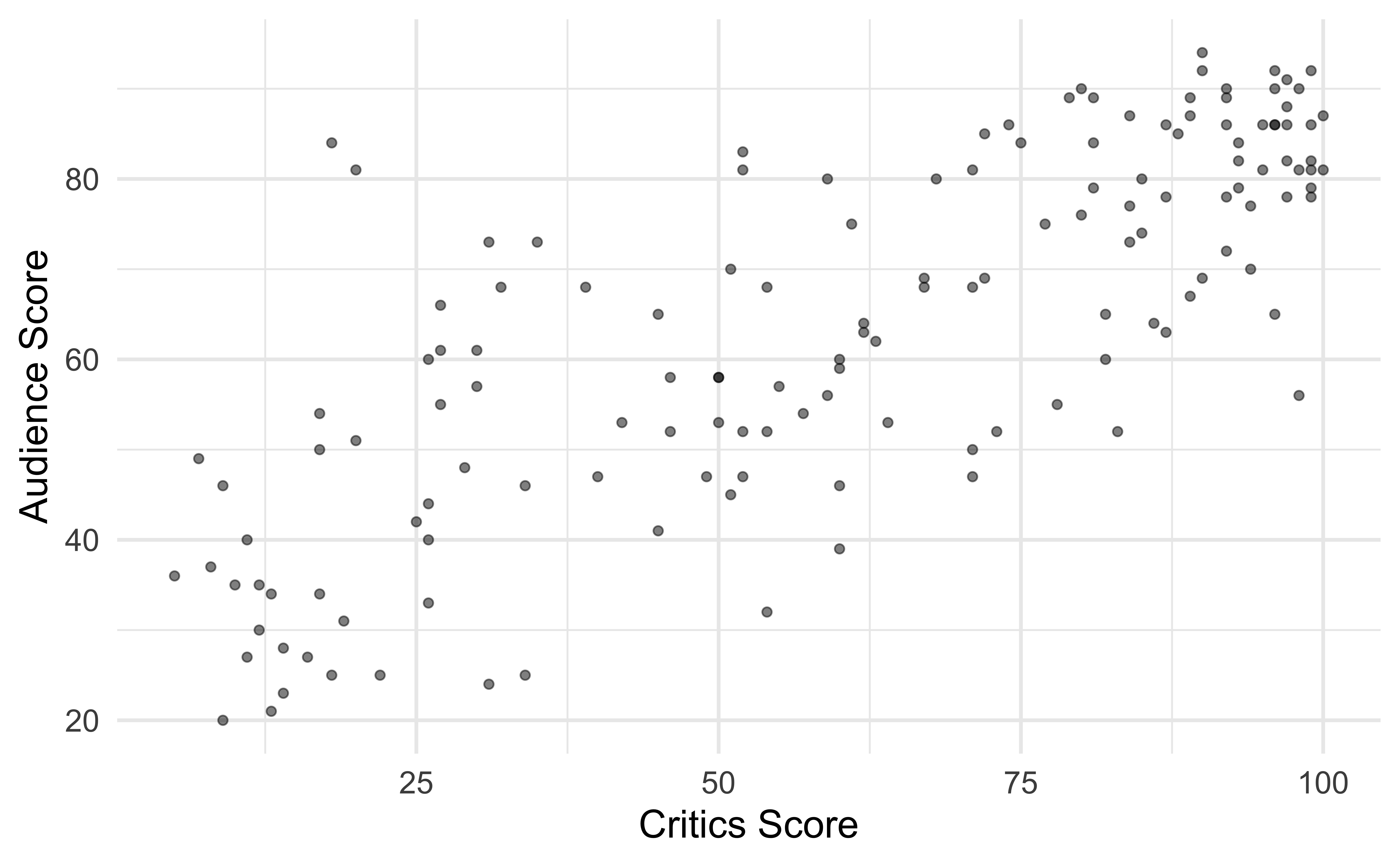
Movie ratings

• Data behind the FiveThirtyEight story Be Suspicious Of Online Movie Ratings, Especially Fandango’s
• In the fivethirtyeight package: fandango
• Contains every film that has at least 30 fan reviews on Fandango, an IMDb score, Rotten Tomatoes critic and user ratings, and Metacritic critic and user scores

Data prep

• Rename Rotten Tomatoes columns as critics and audience
• Rename the dataset as movie_scores

movie_scores <- fandango %>%
  rename(
    critics = rottentomatoes, 
    audience = rottentomatoes_user
  )

Data visualization

Using R for SLR

Step 1: Specify model

linear_reg()

Linear Regression Model Specification (regression)

Computational engine: lm 

Step 2: Set model fitting engine

# #| code-line-numbers: "|2"

linear_reg() %>%
  set_engine("lm") # lm: linear model

Linear Regression Model Specification (regression)

Computational engine: lm 

Step 3: Fit model & estimate parameters

using formula syntax

# #| code-line-numbers: "|3"

linear_reg() %>%
  set_engine("lm") %>%
  fit(audience ~ critics, data = movie_scores)

parsnip model object

Fit time:  4ms 

Call:
stats::lm(formula = audience ~ critics, data = data)

Coefficients:
(Intercept)      critics  
    32.3155       0.5187  

A closer look at model output

movie_fit <- linear_reg() %>%
  set_engine("lm") %>%
  fit(audience ~ critics, data = movie_scores)

movie_fit

parsnip model object

Fit time:  2ms 

Call:
stats::lm(formula = audience ~ critics, data = data)

Coefficients:
(Intercept)      critics  
    32.3155       0.5187  

\[\widehat{\text{audience}} = 32.3155 + 0.5187 \times \text{critics}\]

Note: The intercept is off by a tiny bit from the hand-calculated intercept, this is likely just rounding error in the hand calculation.

The regression output

We’ll focus on the first column for now…

# #| code-line-numbers: "|4"

linear_reg() %>%
  set_engine("lm") %>%
  fit(audience ~ critics, data = movie_scores) %>%
  tidy()

# A tibble: 2 × 5
  term        estimate std.error statistic  p.value
  <chr>          <dbl>     <dbl>     <dbl>    <dbl>
1 (Intercept)   32.3      2.34        13.8 4.03e-28
2 critics        0.519    0.0345      15.0 2.70e-31

Prediction

# #| code-line-numbers: "|2|5"

# create a data frame for a new movie
new_movie <- tibble(critics = 50)

# predict the outcome for a new movie
predict(movie_fit, new_movie)

# A tibble: 1 × 1
  .pred
  <dbl>
1  58.2

Application exercise

📋 github.com/sta210-s22/ae-1-dcbikeshare

followed by a demo of exporting your work and uploading to GradeScope

Recap

• Used tidymodels to fit and summarize regression models in R
• Completed an application exercise on exploratory data analysis and modeling