SLR: Mathematical models for inference

STA 210 - Spring 2022

Dr. Mine Çetinkaya-Rundel

Welcome

Computational setup

# load packages
library(tidyverse)   # for data wrangling and visualization
library(tidymodels)  # for modeling
library(openintro)   # for the duke_forest dataset
library(scales)      # for pretty axis labels
library(knitr)       # for pretty tables
library(kableExtra)  # also for pretty tables

# set default theme and larger font size for ggplot2
ggplot2::theme_set(ggplot2::theme_minimal(base_size = 20))

Recap of last lecture

Data: Duke Forest houses

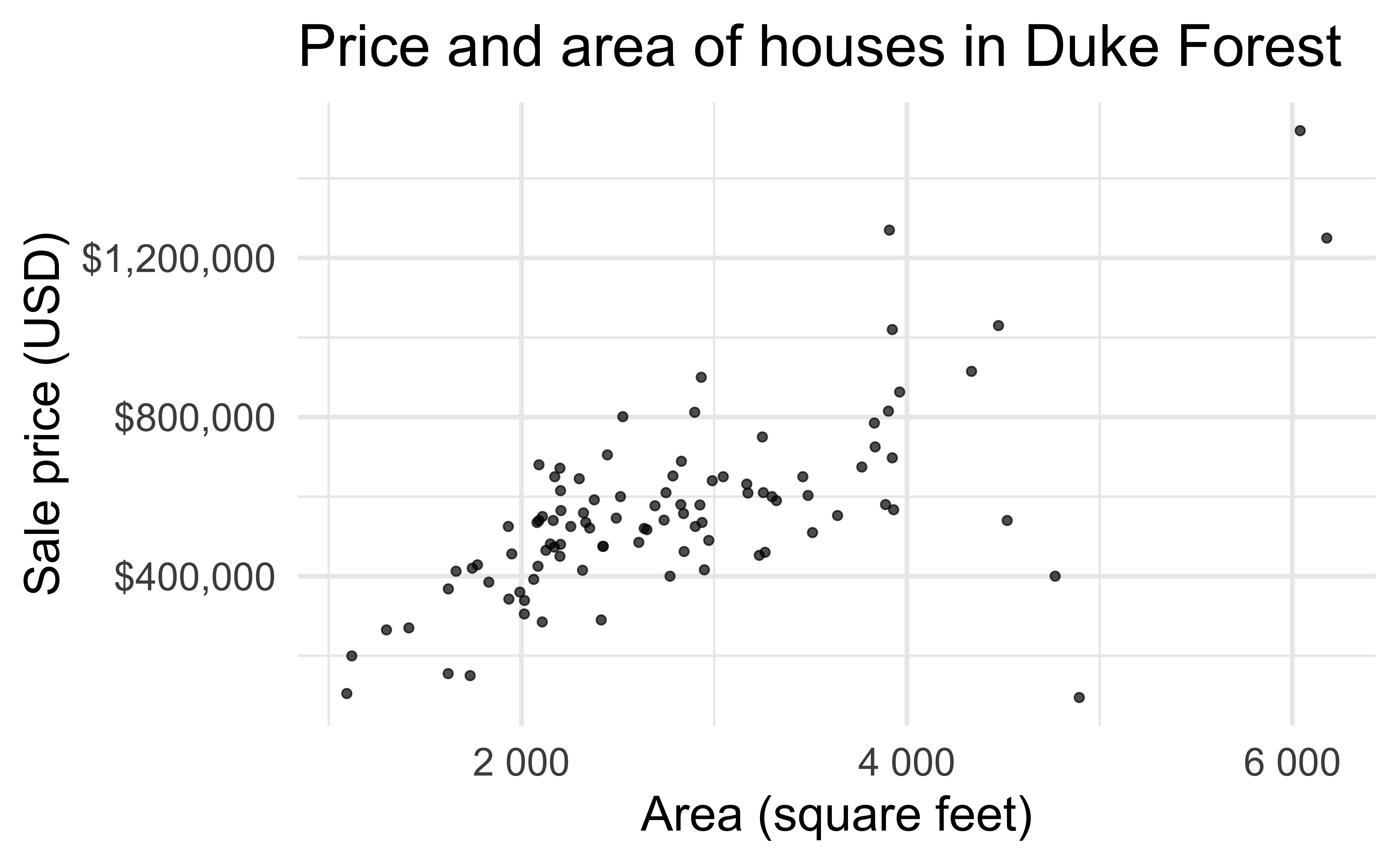
The regression model

df_fit <- linear_reg() %>%
  set_engine("lm") %>%
  fit(price ~ area, data = duke_forest)

tidy(df_fit) %>%
  kable(digits = 2)

term	estimate	std.error	statistic	p.value
(Intercept)	116652.33	53302.46	2.19	0.03
area	159.48	18.17	8.78	0.00

• Intercept: Duke Forest houses that are 0 square feet are expected to sell, on average, for $116,652.
• Slope: For each additional square foot, the model predicts the sale price of Duke Forest houses to be higher, on average, by $159.

Inference for simple linear regression

• Calculate a confidence interval for the slope, \(\beta_1\)

• Conduct a hypothesis test for the interval, \(\beta_1\)

Confidence interval via bootstrapping

• Bootstrap new samples from the original sample
• Fit models to each of the samples and estimate the slope
• Use features of the distribution of the bootstrapped slopes to construct a confidence interval

Bootstrapping pipeline I

# #| code-line-numbers: "|1|3|4"
#| 
set.seed(119)

duke_forest %>%
  specify(price ~ area)

Response: price (numeric)
Explanatory: area (numeric)
# A tibble: 98 × 2
     price  area
     <dbl> <dbl>
 1 1520000  6040
 2 1030000  4475
 3  420000  1745
 4  680000  2091
 5  428500  1772
 6  456000  1950
 7 1270000  3909
 8  557450  2841
 9  697500  3924
10  650000  2173
# … with 88 more rows

Bootstrapping pipeline II

# #| code-line-numbers: "|5"

set.seed(119)

duke_forest %>%
  specify(price ~ area) %>%
  generate(reps = 1000, type = "bootstrap")

Response: price (numeric)
Explanatory: area (numeric)
# A tibble: 98,000 × 3
# Groups:   replicate [1,000]
   replicate   price  area
       <int>   <dbl> <dbl>
 1         1  535000  2334
 2         1  520000  2637
 3         1  540000  2165
 4         1  155000  1620
 5         1  567000  3931
 6         1  420000  1745
 7         1  400000  4769
 8         1  579000  2926
 9         1  615000  2203
10         1 1030000  4475
# … with 97,990 more rows

Bootstrapping pipeline III

# #| code-line-numbers: "|6"

set.seed(119)

duke_forest %>%
  specify(price ~ area) %>%
  generate(reps = 1000, type = "bootstrap") %>%
  fit()

# A tibble: 2,000 × 3
# Groups:   replicate [1,000]
   replicate term      estimate
       <int> <chr>        <dbl>
 1         1 intercept  200401.
 2         1 area          122.
 3         2 intercept  120000.
 4         2 area          156.
 5         3 intercept  190879.
 6         3 area          126.
 7         4 intercept  206842.
 8         4 area          127.
 9         5 intercept  211231.
10         5 area          124.
# … with 1,990 more rows

Bootstrapping pipeline IV

# #| code-line-numbers: "|3"

set.seed(119)

boot_dist <- duke_forest %>%
  specify(price ~ area) %>%
  generate(reps = 1000, type = "bootstrap") %>%
  fit()

Visualize the bootstrap distribution

# #| code-line-numbers: "|2"

boot_dist %>%
  filter(term == "area") %>%
  ggplot(aes(x = estimate)) +
  geom_histogram(binwidth = 10)

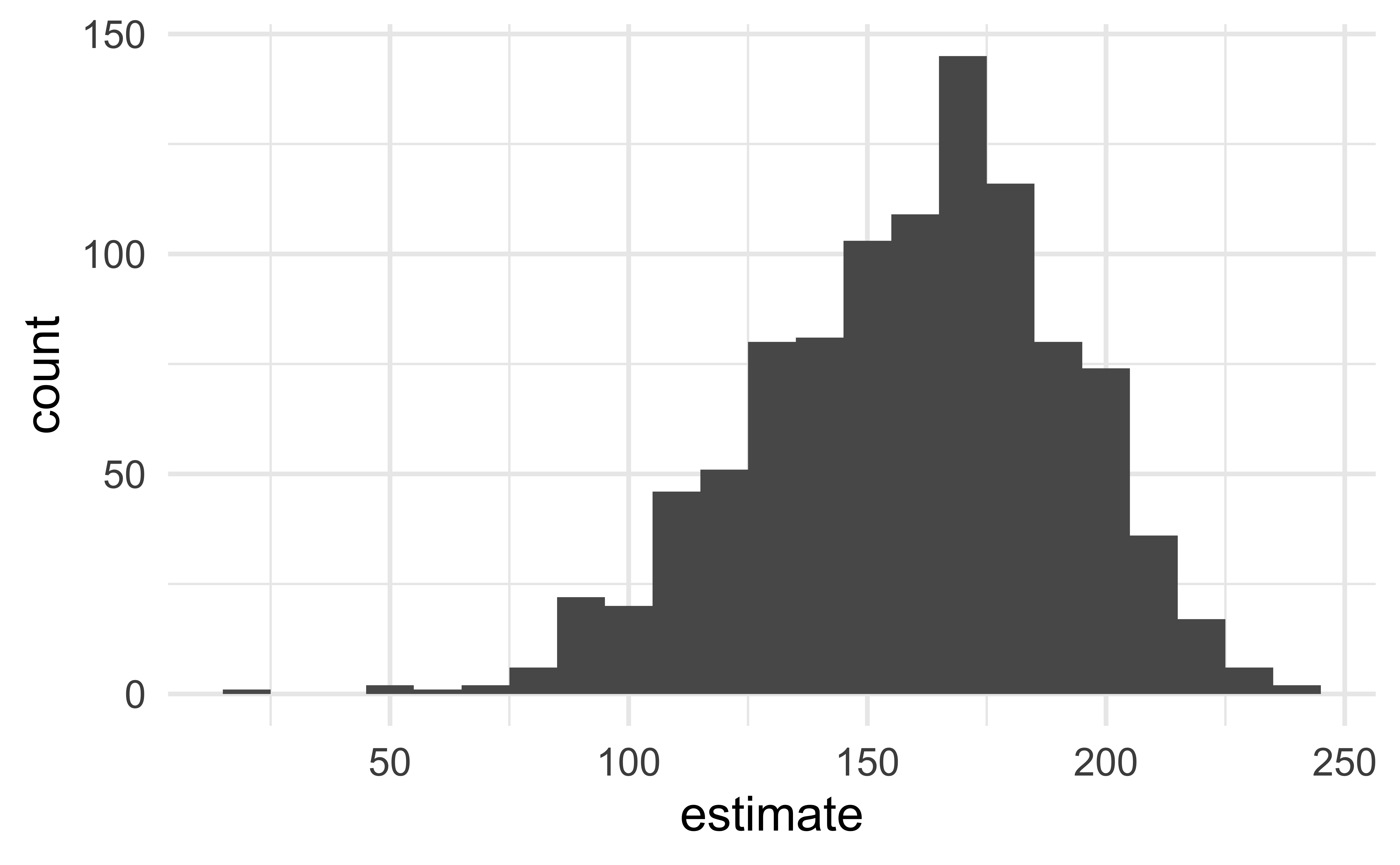
Compute the CI

Two methods:

• Percentile method
• Standard error method

But first…

obs_fit <- duke_forest %>%
  specify(price ~ area) %>%
  fit()

obs_fit

# A tibble: 2 × 2
  term      estimate
  <chr>        <dbl>
1 intercept  116652.
2 area          159.

Percentile method

# #| code-line-numbers: "|4"

boot_dist %>%
  get_confidence_interval(
    level = 0.95,
    type = "percentile",
    point_estimate = obs_fit
  )

# A tibble: 2 × 3
  term      lower_ci upper_ci
  <chr>        <dbl>    <dbl>
1 area          91.0     215.
2 intercept -22046.   289004.

Standard error method

# #| code-line-numbers: "|4"

boot_dist %>%
  get_confidence_interval(
    level = 0.95,
    type = "se",
    point_estimate = obs_fit
  )

# A tibble: 2 × 3
  term      lower_ci upper_ci
  <chr>        <dbl>    <dbl>
1 area          96.1     223.
2 intercept -39805.   273109.

Hypothesis test for the slope

Research question and hypotheses

• “Do the data provide sufficient evidence that \(\beta_1\) (the true slope for the population) is different from 0?”
• Null hypothesis - \(H_0: \beta_1 = 0\), there is no linear relationship between area and price
• Alternative hypothesis - \(H_A: \beta_1 \ne 0\), there is a linear relationship between area and price

Hypothesis testing framework

• Start with a null hypothesis, \(H_0\) that represents the status quo
• Set an alternative hypothesis, \(H_A\) that represents the research question, i.e. what we’re testing for
• Conduct a hypothesis test under the assumption that the null hypothesis is true and calculate a p-value (probability of observed or more extreme outcome given that the null hypothesis is true)
  • if the test results suggest that the data do not provide convincing evidence for the alternative hypothesis, stick with the null hypothesis
  • if they do, then reject the null hypothesis in favor of the alternative

Quantify the variability of the slope

for testing

• Two approaches:
  1. Via simulation (what we’ll review from lab)
  2. Via mathematical models (what we’ll cover in the remainder of class)
• Randomizing to quantify the variability of the slope for the purpose of testing, under the assumption that the null hypothesis is true:
  • Simulate new samples from the original sample via permutation
  • Fit models to each of the samples and estimate the slope
  • Use features of the distribution of the permuted slopes to conduct a hypothesis test

Permutation, described

• Set the null hypothesis to be true, and measure the natural variability in the data due to sampling but not due to variables being correlated by permuting permute one variable to eliminate any existing relationship between the variables
• Each price value is randomly assigned to area of a given house, i.e. area and price are no longer matched for a given house

# A tibble: 98 × 3
   price_Observed price_Permuted  area
            <dbl>          <dbl> <dbl>
 1        1520000         342500  6040
 2        1030000         750000  4475
 3         420000         645000  1745
 4         680000         697500  2091
 5         428500         428500  1772
 6         456000         481000  1950
 7        1270000         610000  3909
 8         557450         680000  2841
 9         697500         485000  3924
10         650000         105000  2173
# … with 88 more rows

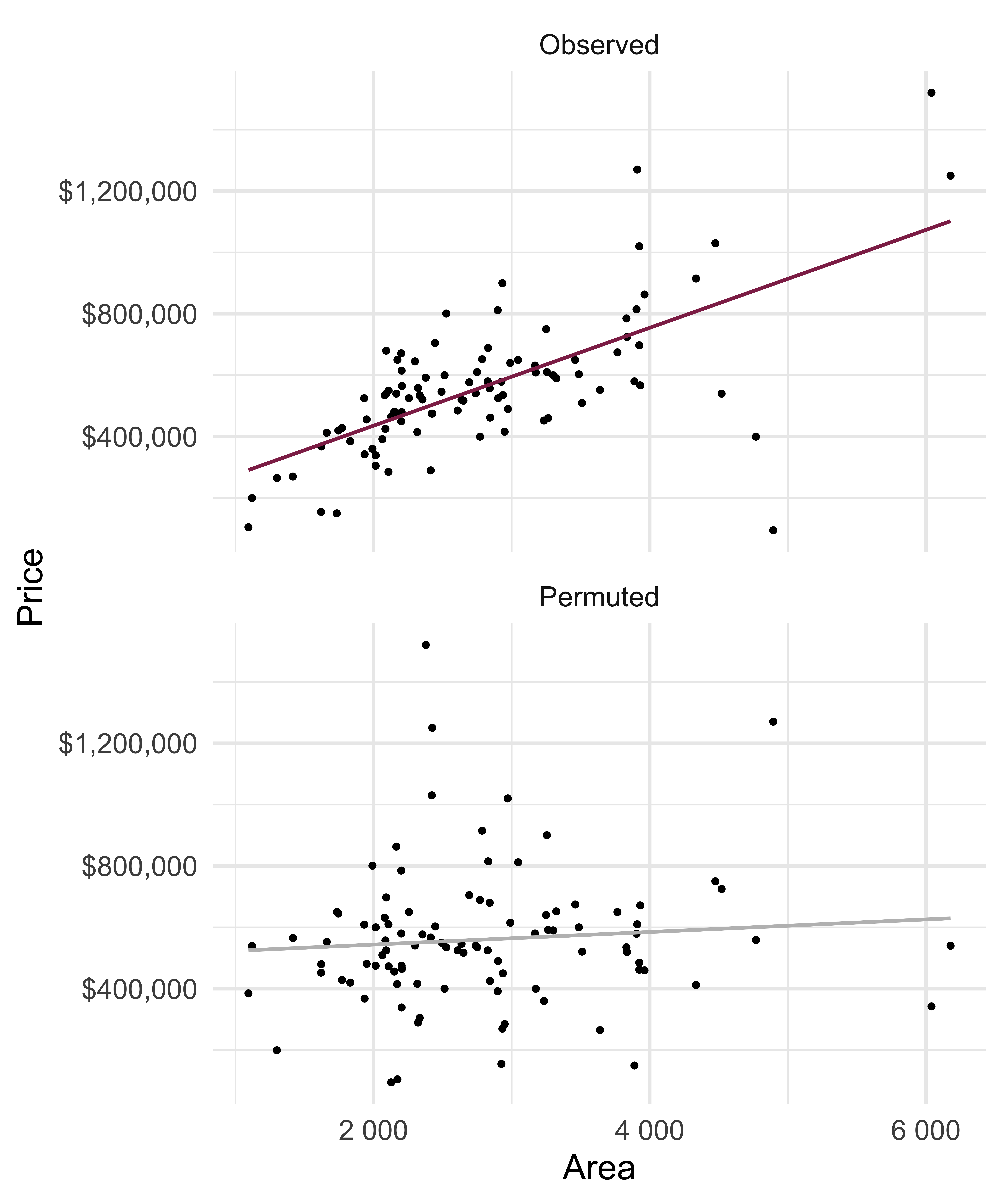
Permutation, visualized

• Each of the observed values for area (and for price) exist in both the observed data plot as well as the permuted price plot
• The permutation removes the linear relationship between area and price

Permutation, repeated

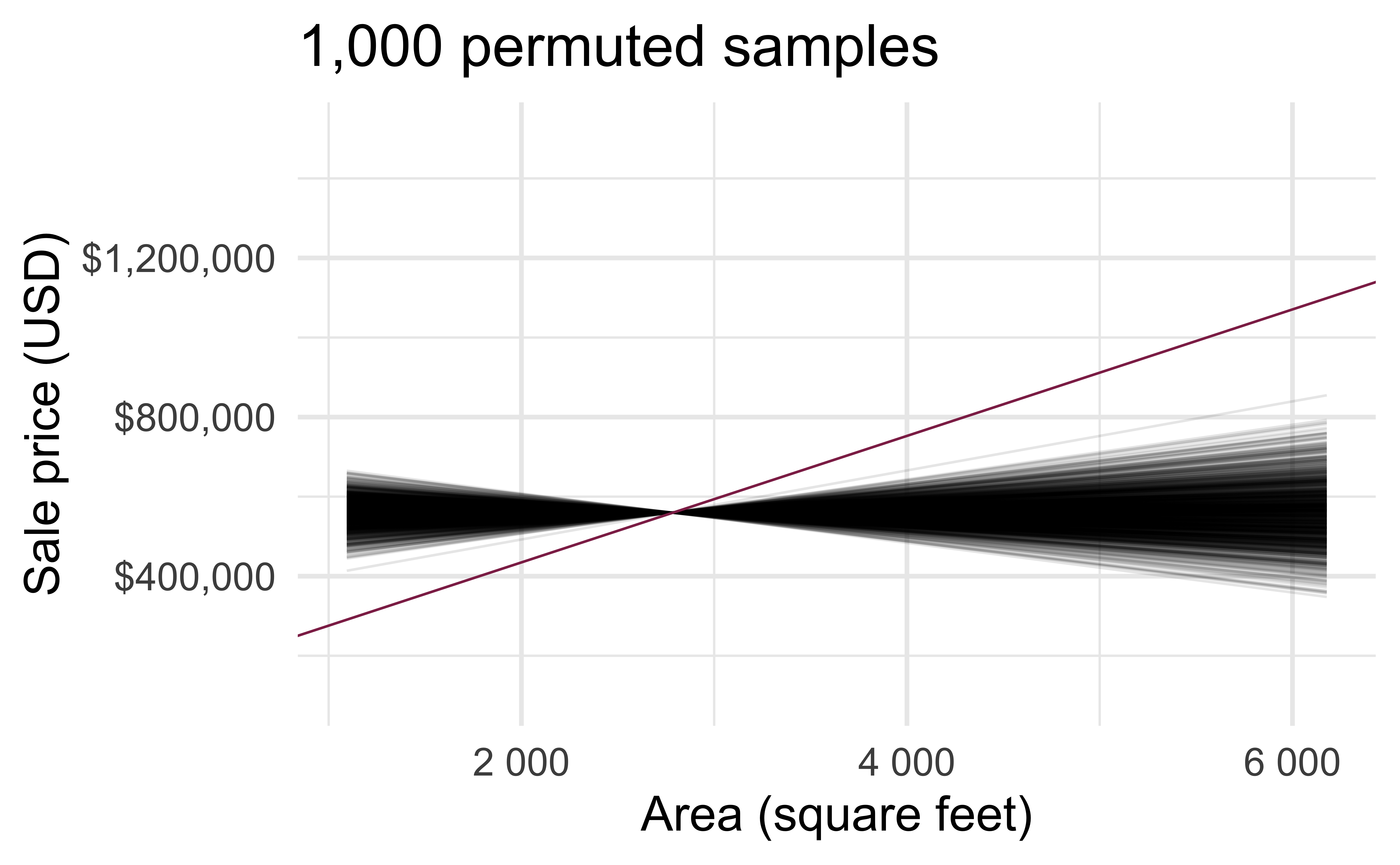
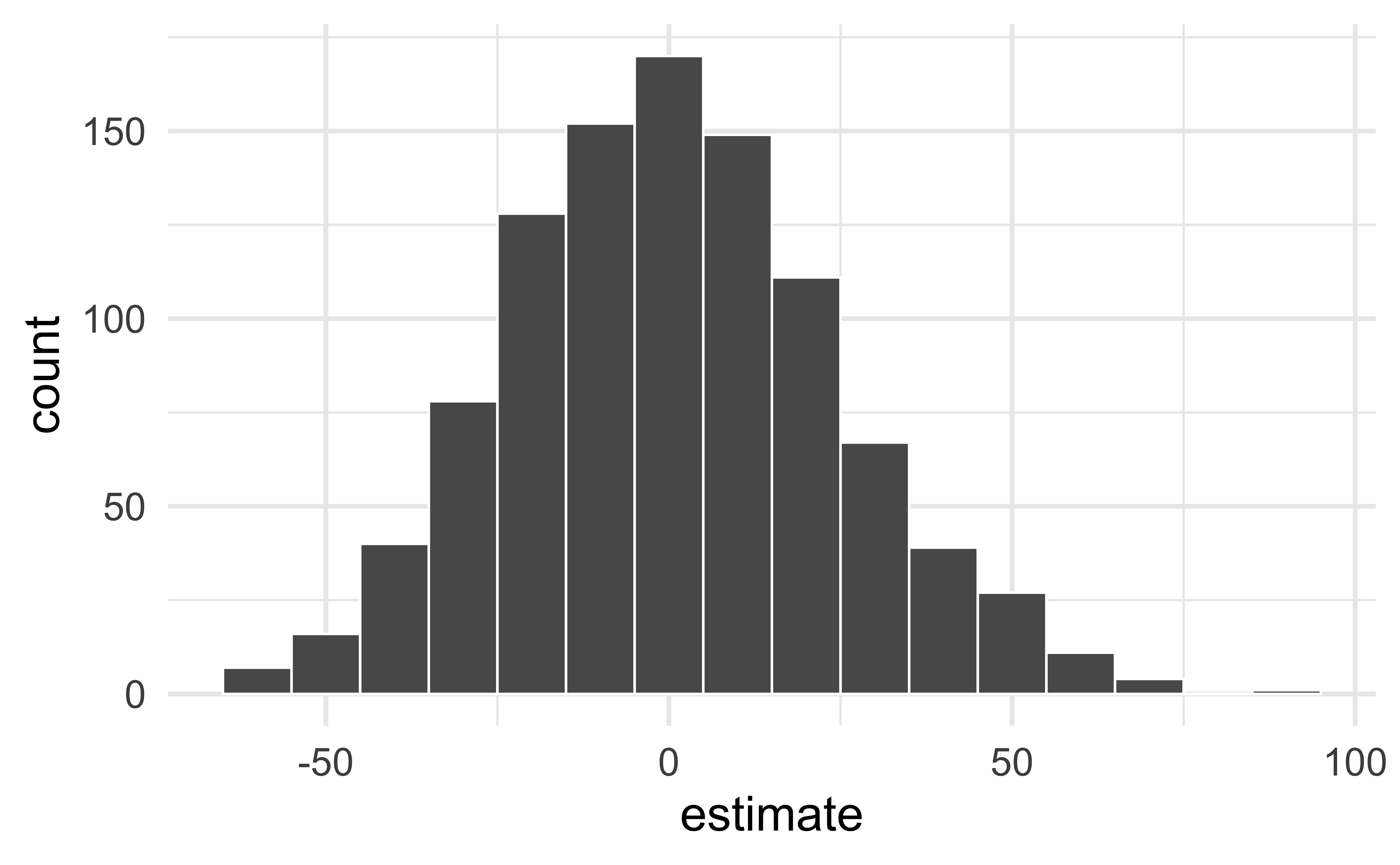
Repeated permutations allow for quantifying the variability in the slope under the condition that there is no linear relationship (i.e., that the null hypothesis is true)

Concluding the hypothesis test

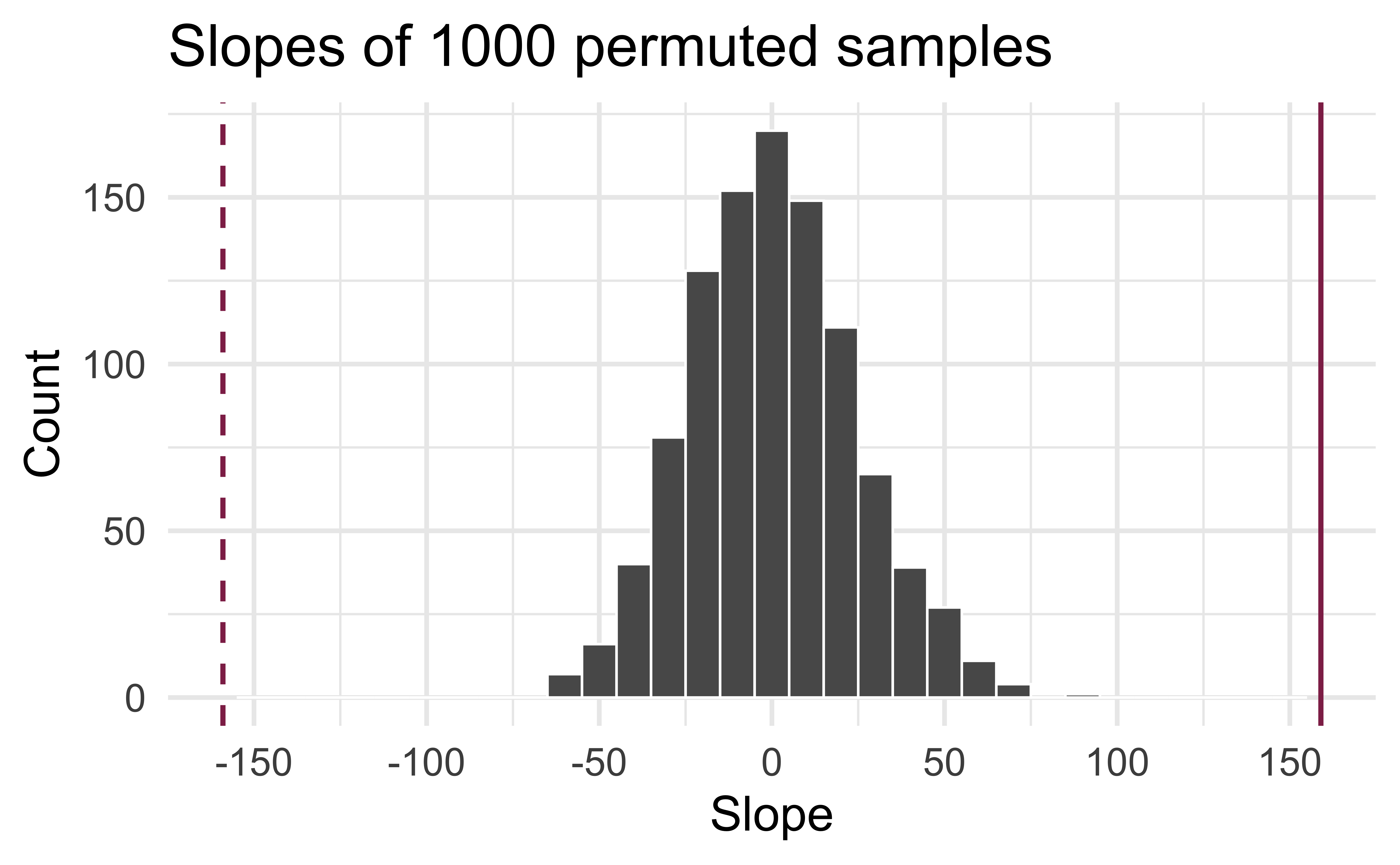
Is the observed slope of \(\hat{\beta_1} = 159\) (or an even more extreme slope) a likely outcome under the null hypothesis that \(\beta = 0\)? What does this mean for our original question: “Do the data provide sufficient evidence that \(\beta_1\) (the true slope for the population) is different from 0?”

Permutation pipeline I

# #| code-line-numbers: "|1|3|4"
#| 
set.seed(1125)

duke_forest %>%
  specify(price ~ area)

Response: price (numeric)
Explanatory: area (numeric)
# A tibble: 98 × 2
     price  area
     <dbl> <dbl>
 1 1520000  6040
 2 1030000  4475
 3  420000  1745
 4  680000  2091
 5  428500  1772
 6  456000  1950
 7 1270000  3909
 8  557450  2841
 9  697500  3924
10  650000  2173
# … with 88 more rows

Permutation pipeline II

# #| code-line-numbers: "|5"

set.seed(1125)

duke_forest %>%
  specify(price ~ area) %>%
  hypothesize(null = "independence")

Response: price (numeric)
Explanatory: area (numeric)
Null Hypothesis: independence
# A tibble: 98 × 2
     price  area
     <dbl> <dbl>
 1 1520000  6040
 2 1030000  4475
 3  420000  1745
 4  680000  2091
 5  428500  1772
 6  456000  1950
 7 1270000  3909
 8  557450  2841
 9  697500  3924
10  650000  2173
# … with 88 more rows

Permutation pipeline III

# #| code-line-numbers: "|6"

set.seed(1125)

duke_forest %>%
  specify(price ~ area) %>%
  hypothesize(null = "independence") %>%
  generate(reps = 1000, type = "permute")

Response: price (numeric)
Explanatory: area (numeric)
Null Hypothesis: independence
# A tibble: 98,000 × 3
# Groups:   replicate [1,000]
     price  area replicate
     <dbl> <dbl>     <int>
 1  465000  6040         1
 2  481000  4475         1
 3 1020000  1745         1
 4  520000  2091         1
 5  592000  1772         1
 6  650000  1950         1
 7  473000  3909         1
 8  705000  2841         1
 9  785000  3924         1
10  671500  2173         1
# … with 97,990 more rows

Permutation pipeline IV

# #| code-line-numbers: "|7"

set.seed(1125)

duke_forest %>%
  specify(price ~ area) %>%
  hypothesize(null = "independence") %>%
  generate(reps = 1000, type = "permute") %>%
  fit()

# A tibble: 2,000 × 3
# Groups:   replicate [1,000]
   replicate term       estimate
       <int> <chr>         <dbl>
 1         1 intercept 553355.  
 2         1 area           2.35
 3         2 intercept 635824.  
 4         2 area         -27.3 
 5         3 intercept 536072.  
 6         3 area           8.57
 7         4 intercept 598649.  
 8         4 area         -13.9 
 9         5 intercept 556202.  
10         5 area           1.33
# … with 1,990 more rows

Permutation pipeline V

# #| code-line-numbers: "|3"

set.seed(1125)

null_dist <- duke_forest %>%
  specify(price ~ area) %>%
  hypothesize(null = "independence") %>%
  generate(reps = 1000, type = "permute") %>%
  fit()

Visualize the null distribution

# #| code-line-numbers: "|2"

null_dist %>%
  filter(term == "area") %>%
  ggplot(aes(x = estimate)) +
  geom_histogram(binwidth = 10, color = "white")

Reason around the p-value

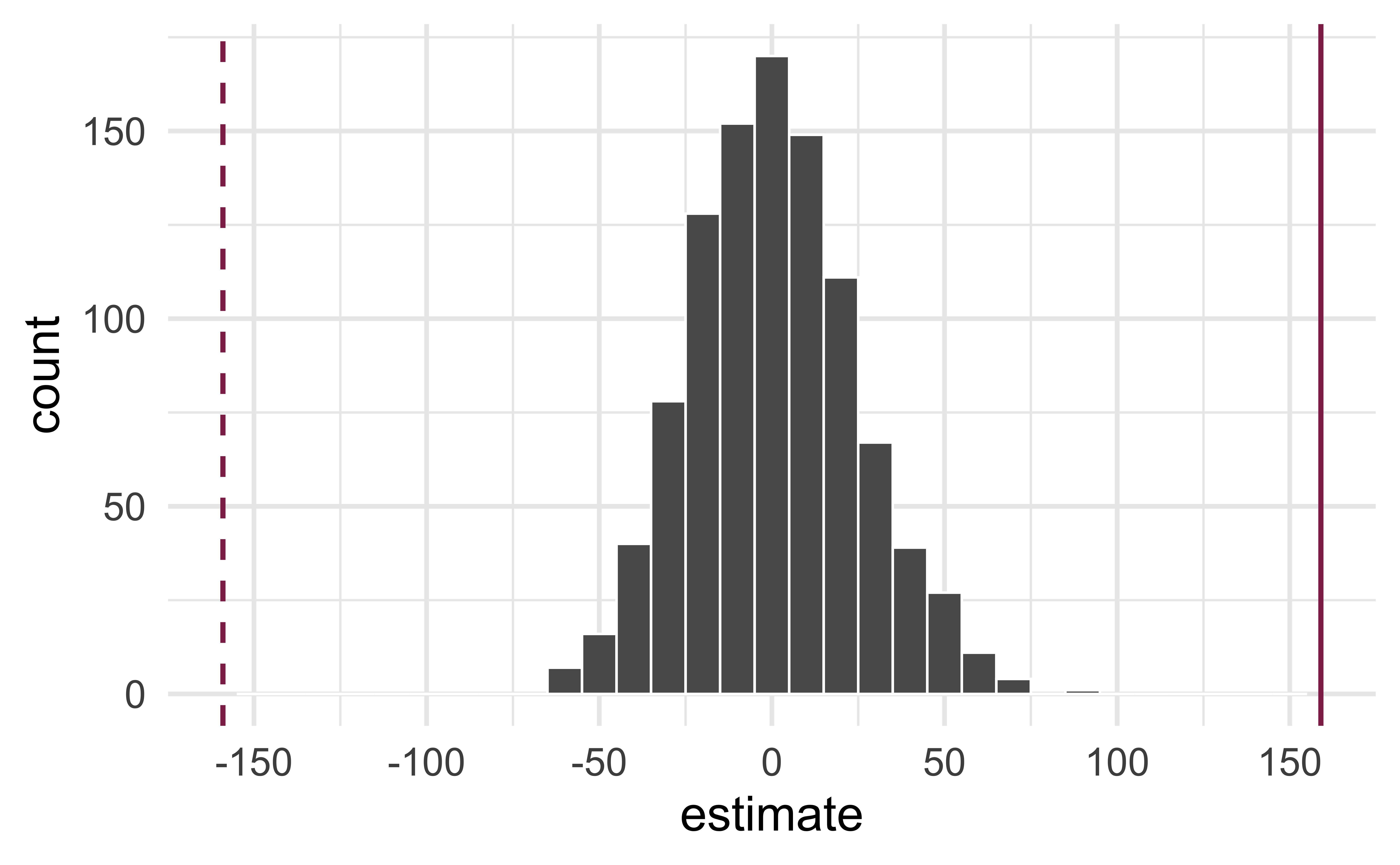
In a world where the there is no relationship between the area of a Duke Forest house and in its price (\(\beta_1 = 0\)), what is the probability that we observe a sample of 98 houses where the slope fo the model predicting price from area is 159 or even more extreme?

Compute the p-value

What does this warning mean?

get_p_value(
  null_dist,
  obs_stat = obs_fit,
  direction = "two-sided"
)

Warning: Please be cautious in reporting a p-value of 0. This result is an
approximation based on the number of `reps` chosen in the `generate()` step. See
`?get_p_value()` for more information.

Warning: Please be cautious in reporting a p-value of 0. This result is an
approximation based on the number of `reps` chosen in the `generate()` step. See
`?get_p_value()` for more information.

# A tibble: 2 × 2
  term      p_value
  <chr>       <dbl>
1 area            0
2 intercept       0

Mathematical models for inference

The regression model, revisited

df_fit <- linear_reg() %>%
  set_engine("lm") %>%
  fit(price ~ area, data = duke_forest)

tidy(df_fit) %>%
  kable(digits = 3)

term	estimate	std.error	statistic	p.value
(Intercept)	116652.325	53302.463	2.188	0.031
area	159.483	18.171	8.777	0.000

HT and CI, recapped

• Hypothesis test:

  • Do the data provide sufficient evidence that \(\beta_1\) (the true slope for the population) is different from 0?
  • Null hypothesis - \(H_0: \beta_1 = 0\), there is no linear relationship between area and price.
  • Alternative hypothesis - \(H_A: \beta_1 \ne 0\), there is a linear relationship between area and price.

• Confidence interval: Provide a plausible range of values for \(\beta_1\) at a given confidence level.

HT and CI, revisited

• Earlier we computed a CI and conducted a HT via simulation:
  • CI: Bootstrap the observed sample to simulate the distribution of the slope
  • HT: Permute the observed sample to simulate the distribution of the slope under the assumption that the null hypothesis is true
• Now we’ll do these based on theoretical results, i.e., by using the Central Limit Theorem to define the distribution of the slope and use features (shape, center, spread) of this distribution to compute bounds of the CI and the p-value for the HT

Mathematical representation of the model

\[ \begin{aligned} Y &= Model + Error \\ &= f(X) + \epsilon \\ &= \mu_{Y|X} + \epsilon \\ &= \beta_0 + \beta_1 X + \epsilon \end{aligned} \]

where the errors are independent and normally distributed:

• independent: Knowing the error term for one observation doesn’t tell you anything about the error term for another observation
• normally distributed: \(\epsilon \sim N(0, \sigma_\epsilon^2)\)

Mathematical representation, visualized

\[ Y|X \sim N(\beta_0 + \beta_1 X, \sigma_\epsilon^2) \]

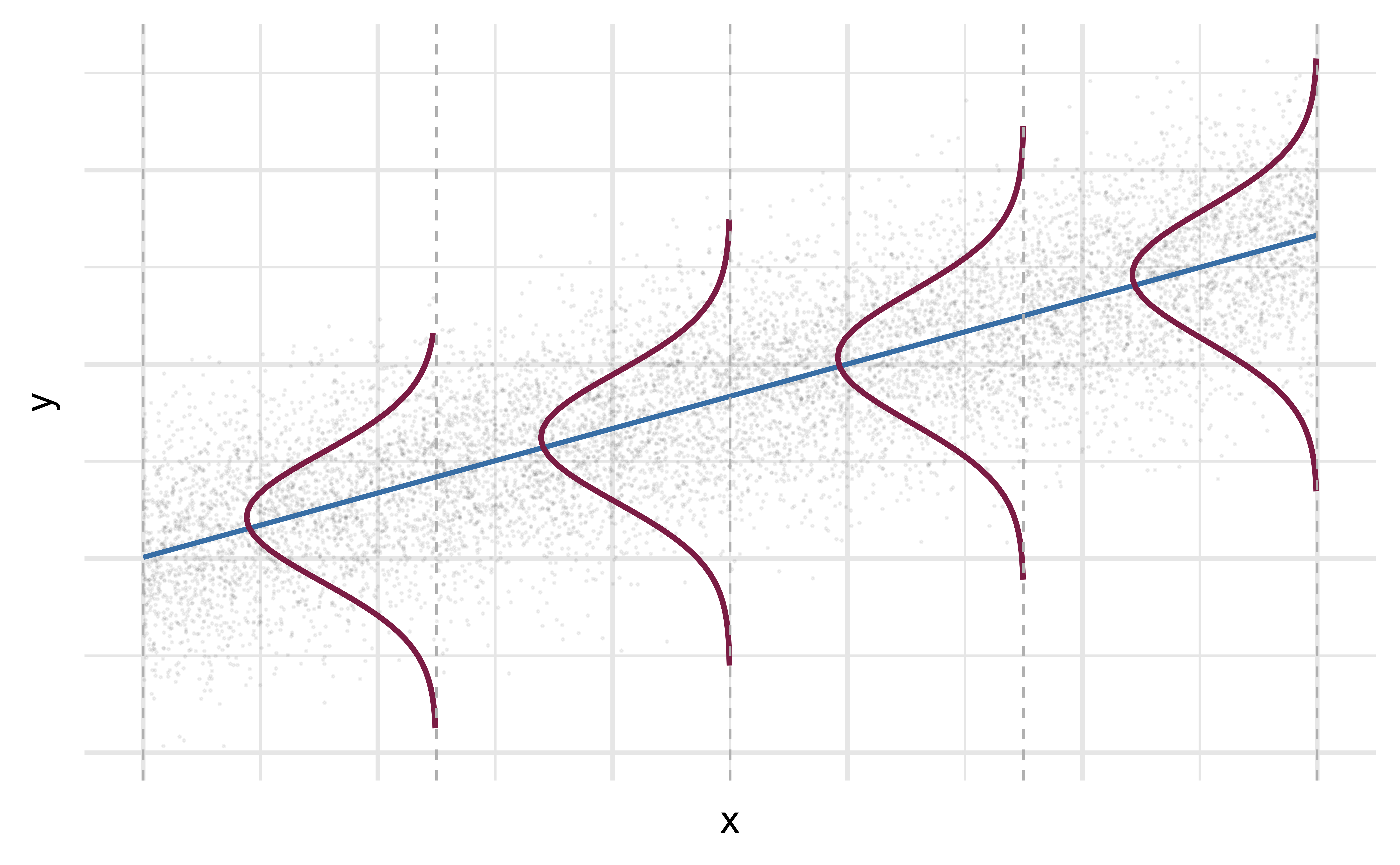
• Mean: \(\beta_0 + \beta_1 X\), the predicted value based on the regression model
• Variance: \(\sigma_\epsilon^2\), constant across the range of \(X\)
  • How do we estimate \(\sigma_\epsilon^2\)?

Regression standard error

Once we fit the model, we can use the residuals to estimate the regression standard error (the spread of the distribution of the response, for a given value of the predictor variable):

\[ \hat{\sigma}_\epsilon = \sqrt{\frac{\sum_\limits{i=1}^n(y_i - \hat{y}_i)^2}{n-2}} = \sqrt{\frac{\sum_\limits{i=1}^ne_i^2}{n-2}} \]

1. Why divide by \(n - 2\)?
2. Why do we care about the value of the regression standard error?

Standard error of \(\hat{\beta}_1\)

\[ SE_{\hat{\beta}_1} = \hat{\sigma}_\epsilon\sqrt{\frac{1}{(n-1)s_X^2}} \]

or…

term	estimate	std.error	statistic	p.value
(Intercept)	116652.33	53302.46	2.19	0.03
area	159.48	18.17	8.78	0.00