library(tidyverse)
library(tidymodels)
library(knitr)
library(Stat2Data)
library(rms)
library(nnet)AE 12: Exam 3 Review
Important
Go to the course GitHub organization and locate the repo titled ae-12-exam-3-review-YOUR_GITHUB_USERNAME to get started.
Introduction
Packages
Data
As part of a study of the effects of predatory intertidal crab species on snail populations, researchers measured the mean closing forces and the propodus heights of the claws on several crabs of three species.

claws <- read_csv(here::here("ae", "data/claws.csv"))We will use the following variables:
force: Closing force of claw (newtons)height: Propodus height (mm)species: Crab species - Cp(Cancer productus), Hn (Hemigrapsus nudus), Lb(Lophopanopeus bellus)lb: 1 if Lophopanopeus bellus species, 0 otherwisehn: 1 if Hemigrapsus nudus species, 0 otherwisecp: 1 if Cancer productus species, 0 otherwiseforce_cent: mean centered forceheight_cent: mean centered height
Before we get started, let’s make the categorical and indicator variables factors.
claws <- claws %>%
  mutate(
    species = as_factor(species),
    lb = as_factor(lb),
    hn = as_factor(hn),
    cp = as_factor(cp)
  )
Part 1
Probabilities vs. odds vs. log-odds
Why we use log-odds as response variable: https://sta210-s22.github.io/website/slides/lec-18.html#/do-teenagers-get-7-hours-of-sleep
Exercise 1
Fill in the blanks:
- Use log-odds to fit the model (outcome)
- Use odds to interpret model results
- Use probabilities to make predictions for individual observations and ultimately to make classification decisions
Exercise 2
Suppose we want to use force to determine whether or not a crab is from the Lophopanopeus bellus (Lb) species. Why should we use a logistic regression model for this analysis?
claws %>%
  distinct(lb)
# A tibble: 2 × 1
lb
<fct>
1 0
2 1 Exercise 3
We will use the mean-centered variables for force in the model. The model output is below. Write the equation of the model produced by R. Don’t forget to fill in the blanks for ….
| term | estimate | std.error | statistic | p.value | conf.low | conf.high |
|---|---|---|---|---|---|---|
| (Intercept) | -0.798 | 0.358 | -2.233 | 0.026 | -1.542 | -0.123 |
| force_cent | 0.043 | 0.039 | 1.090 | 0.276 | -0.034 | 0.123 |
Let \(\pi\) be probability that a crab is from Lb species.
\[ \log\Big(\frac{\hat{\pi}}{1 - \hat{\pi}}\Big) = -0.798 + 0.043 * force\_cent \]
Exercise 4
Interpret the intercept in the context of the data.
mean_force <- round(mean(claws$force), 2)For crabs with average closing force (12.13 newtons), we expect odds of the crab being Lophopanopeus bellus is 0.45 (exp(-0.798)).
Exercise 5
Interpret the effect of force in the context of the data.
When x goes up by 1 unit, we expect y to change by (slope) units.
For each additional unit increase in closing force, the odds of crab being from lb species multiplies on average by a factor of 1.0439379.
Exercise 6
Now let’s consider adding height_cent to the model. Fit the model that includes height_cent. Then use AIC to choose the model that best fits the data.
lb_fit_2 <- logistic_reg() %>%
  set_engine("glm") %>%
  fit(lb ~ force_cent + height_cent, data = claws)

tidy(lb_fit_2, conf.int = TRUE)
# A tibble: 3 × 7
term estimate std.error statistic p.value conf.low conf.high
<chr> <dbl> <dbl> <dbl> <dbl> <dbl> <dbl>
1 (Intercept) -1.13 0.463 -2.44 0.0146 -2.17 -0.306
2 force_cent 0.211 0.0925 2.28 0.0227 0.0563 0.424
3 height_cent -0.895 0.398 -2.25 0.0245 -1.82 -0.234glance(lb_fit_1)$AIC[1] 50.19535glance(lb_fit_2)$AIC[1] 44.11812Exercise 7
What do the following mean in the context of this data. Explain and calculate them.
- Sensitivity: P(predict lb | actual lb) = 6 / 12
- Specificity: P(predict not lb | actual not lb) = 4/ 26
- Negative predictive power: P(actual not lb | predict not lb) = 22 / 28
- Positive predictive power: P(actual lb | predict lb) = 6 / 10
| Actual | Predict lb | Predict not lb | TOTAL predicted |
|---|---|---|---|
| Lb | 6 | 6 | 12 |
| Not lb | 4 | 22 | 26 |
| TOTAL actual | 10 | 28 | 38 |
Part 2
Let’s extend the model to use force and height to predict the species (Hn, Cp, and Lb). The model output is below:
species_fit <- multinom_reg() %>%
  set_engine("nnet") %>%
  fit(species ~ force_cent + height_cent, data = claws)

species_fit <- repair_call(species_fit, data = claws)

tidy(species_fit, conf.int = TRUE)
# A tibble: 6 × 8
y.level term estimate std.error statistic p.value conf.low conf.high
<chr> <chr> <dbl> <dbl> <dbl> <dbl> <dbl> <dbl>
1 Lb (Intercept) 1.21 1.11 1.10 0.273 -0.956 3.38
2 Lb force_cent 0.589 0.204 2.88 0.00393 0.189 0.989
3 Lb height_cent -1.08 0.514 -2.11 0.0352 -2.09 -0.0753
4 Cp (Intercept) 1.19 1.10 1.08 0.281 -0.974 3.36
5 Cp force_cent 0.494 0.197 2.51 0.0120 0.109 0.879
6 Cp height_cent -0.180 0.475 -0.380 0.704 -1.11 0.750 Exercise 8
Write the equation of the model.
\[\log\Big(\frac{\hat{\pi}_{Hn}}{\hat{\pi}_{Cp}}\Big) = \]
\[\log\Big(\frac{\hat{\pi}_{Lb}}{\hat{\pi}_{Cp}}\Big) = \]
Exercise 9
Interpret the intercept for the odds a crab is Hn vs. Cp species.
Interpret the effect of force on the odds a crab is Lb vs. Cp species.
Exercise 10
Interpret the effect of force on the odds a crab is in the Hn vs. Lb species.
CAUTION: We can write an interpretation based on the estimated coefficients; however, we can’t make any inferential conclusions for this question based on the current model. We would need to refit the model with Lb as the baseline category to do so.
Exercise 11
Conditions for multinomial logistic (and logistic models as well):
- Independence:
- Randomness:
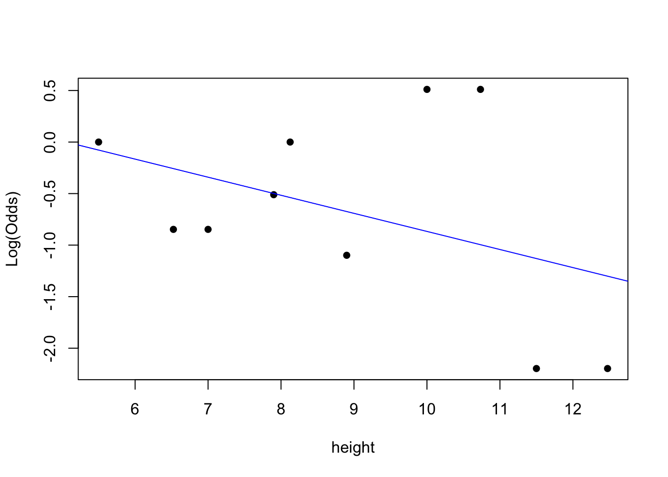
- Linearity:
emplogitplot1(lb ~ force, data = claws, ngroups = 10)
emplogitplot1(lb ~ height, data = claws, ngroups = 10)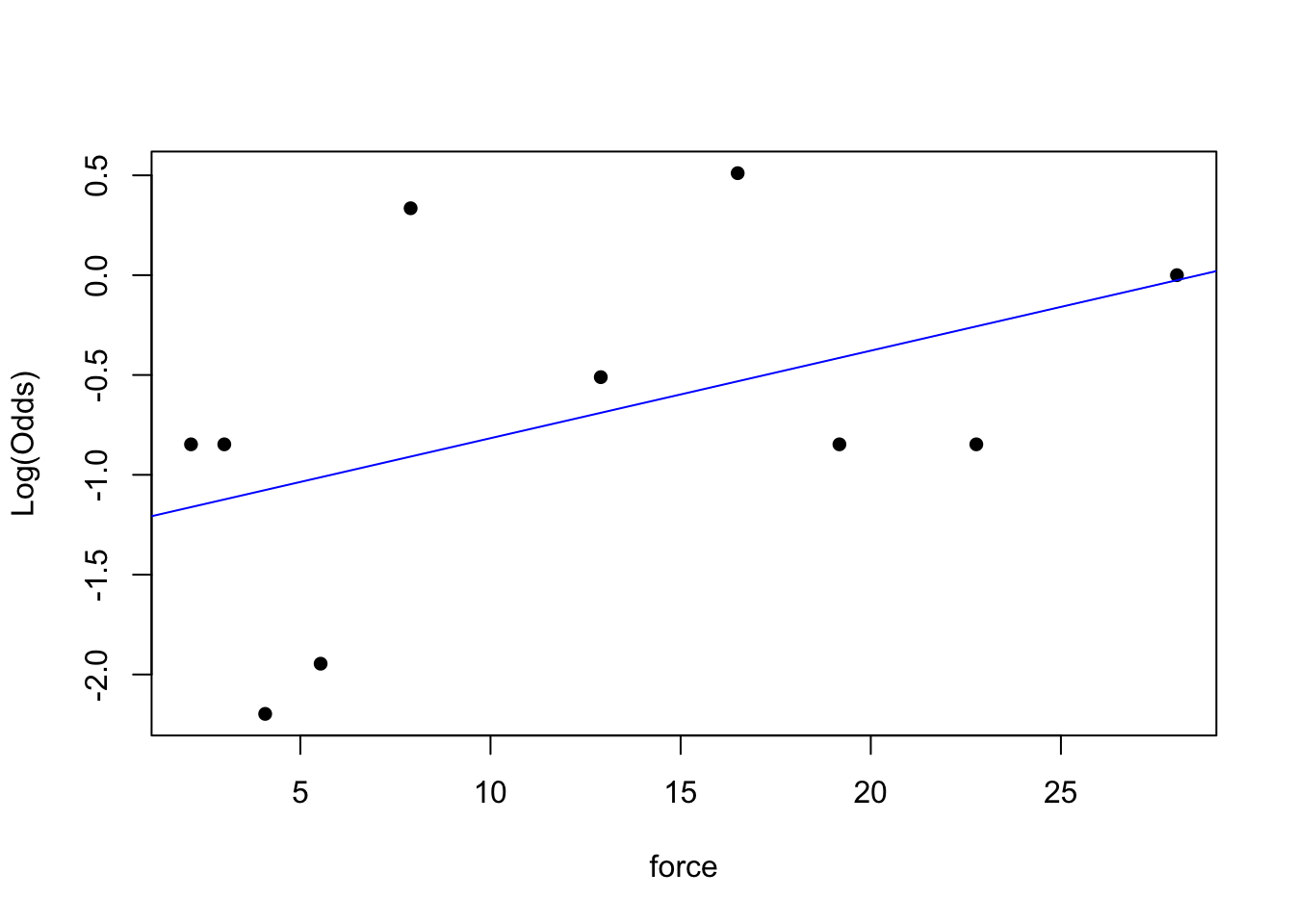
# add code here for other species here# add code here for other species herePart 3
Checking for multicollinearity in logistic and multinomial logistic
Similar to multiple linear regression, we can also check for multicollinearity in logistic and multinomial logistic models.
- Use the
viffunction to check for multicollinearity in logistic regression.
- The
viffunction doesn’t work for the multinomial logistic regression models, so we can look at a correlation matrix of the predictors as a way to assess if the predictors are highly correlated: